https://savedforlater.dev/feed.xmlSaved for Later2026-07-22T20:20:51.041Zhttps://github.com/jacobwgillespie/saved-for-later<![CDATA[Late.sh – a command-line Clubhouse for computer people]]>https://late.sh/2026-07-22T02:32:30.000ZComments]]><![CDATA[Let Tom Hiddleston be your guide to Pompeii's final day]]>https://arstechnica.com/science/2026/07/tom-hiddleston-tracks-possible-pompeii-survivors-in-new-docuseries/2026-07-21T18:17:55.000ZWhen Mount Vesuvius erupted in 79 CE, it spewed molten rock, pumice, and hot ash over the cities of Pompeii and Herculaneum, killing thousands of people. It's one of the most famous natural disasters in human history, so naturally there have been countless documentaries about Pompeii (and at least one popular song). But only one features actor Tom Hiddleston taking on the role of a "time detective" to bring the people of Pompeii to vivid life. That would be National Geographic's new three-part docuseries, Pompeii: Out of Time.
The Marvel connection made Out of Time happen. Executive producer Kevin Wright was also a producer on the Disney+ series Loki, which included a scene where Hiddleston's Loki travels through time to visit Pompeii. Hiddleston also studied classics at Cambridge University and had visited the Pompeii archaeological site as a teenager, which the Marvel star attributes to indirectly influencing his career path into acting.
"There is just a passion to the way Tom tells stories that's infectious," Wright told Ars. "We knew that if we could capture that and put it into [the series], it might interest people who wouldn't normally want to watch a documentary about Pompeii. "
]]><![CDATA[Jack Dorsey launches Buzz to combine team chat, AI agents and Git hosting]]>https://runtimewire.com/article/jack-dorsey-block-buzz-team-chat-ai-agents-git2026-07-21T17:14:06.000ZComments]]><![CDATA[Stop Using OpenCode]]>https://wren.wtf/shower-thoughts/stop-using-opencode/2026-07-20T12:45:55.000ZComments]]><![CDATA[How Version Control Will Evolve for the Agent Boom]]>https://entire.io/blog/how-version-control-will-evolve-for-the-agent-boom2026-07-09T12:20:41.000ZComments]]><![CDATA[Kani: A Model Checker for Rust]]>https://arxiv.org/abs/2607.015042026-07-06T15:53:24.000ZComments]]><![CDATA[Show HN: ZeroFS – A log-structured filesystem for S3]]>https://www.zerofs.net/2026-07-02T13:41:11.000ZComments]]><![CDATA[Accelerate your infrastructure deployments by up to 4x with AWS CloudFormation Express mode]]>https://aws.amazon.com/blogs/aws/accelerate-your-infrastructure-deployments-by-up-to-4x-with-aws-cloudformation-express-mode/2026-06-30T21:30:33.000ZToday, we’re announcing AWS CloudFormation Express mode, a new deployment mode that accelerates deployments for developers and AI tools iterating on infrastructure. Express mode accelerates deployments by completing when CloudFormation confirms resource configuration is applied, rather than waiting for extended stabilization checks. This reduces deployment time by up to 4 times for iterative development workflows and production scenarios.
How it works Every CloudFormation deployment performs stabilization checks after resource configuration is applied. These checks serve an important purpose when you need to confirm resources can serve traffic before shifting load.
However, many workflows do not require full stabilization to proceed. Express mode benefits two primary use cases: iterative development workflows and production scenarios where you are comfortable with eventual stabilization. These use cases include iterating on infrastructure configurations during development, testing individual components of your application, and AI-assisted infrastructure development that benefits from sub-minute feedback loops.
With Express mode, CloudFormation completes deployments when resource configuration is applied, without waiting for stabilization checks. Resources continue becoming operational in the background. CloudFormation automatically retries dependent resources that encounter transient failures during provisioning within the same stack, without requiring any customer intervention. This built-in resilience handles timing issues between resources as they stabilize. Express mode changes when the deployment completes, not how resources are provisioned.
For example, when I create an Amazon Simple Queue Service (SQS) queue with a dead letter queue (DLQ), Standard mode takes 64 seconds, but Express mode completes in up to 10 seconds. In the case of deleting an AWS Lambda function with network interface attachment, Standard mode takes 20–30 minutes, but Express mode completes in up to 10 seconds based on my benchmarking test.
Get started with CloudFormation Express mode When you create a CloudFormation stack in the AWS Management Console, choose Enable in the Express mode under Stack deployment options.
Activate Express mode by setting the --deployment-config parameter to EXPRESS when creating, updating, or deleting stacks. No template changes are required. Express mode disables rollback by default for the fastest iteration experience. To re-enable rollback, set disableRollback to false in the deployment-config for production environments, or implement monitoring/cleanup mechanisms for failed deployments.
For example, use the Express mode when you build infrastructure incrementally, adding resources one at a time. Ensure your IAM role templates follow the principle of least privilege.
For AWS CDK, activate Express mode with the cdk deploy --express command when you deploy your CDK stack. This command retrieves your generated CloudFormation template and deploys it through the CloudFormation Express mode, which provisions your resources as part of a CloudFormation stack.
Express mode works with all existing CloudFormation templates and supports all CloudFormation features including change sets and nested stacks. When you enable Express mode on a parent stack, all nested stacks also use Express mode. If you need resources to be fully operational before proceeding with traffic or testing, continue using the default deployment behavior, which performs stabilization checks before completing.
Now available AWS CloudFormation Express mode is available today in all AWS commercial Regions at no additional cost. For Regional availability and a future roadmap, visit the AWS Capabilities by Region. If you want to call APIs, search documentation, find regional availability, and check troubleshooting about this new feature, try using the AWS MCP Server and plugins with your preferred AI tool. To learn more, visit the CloudFormation documentation.
Start accelerating your deployments today, and send feedback to AWS re:Post for AWS CloudFormation or through your usual AWS Support contacts.
]]><![CDATA[OAuth for all]]>https://blog.cloudflare.com/oauth-for-all/2026-06-25T02:18:10.000ZComments]]><![CDATA[Run isolated sandboxes with full lifecycle control: AWS Lambda introduces MicroVMs]]>https://aws.amazon.com/blogs/aws/run-isolated-sandboxes-with-full-lifecycle-control-aws-lambda-introduces-microvms/2026-06-22T22:40:07.000ZToday, we are announcing AWS Lambda MicroVMs, a new serverless compute primitive within AWS Lambda that lets you run code generated by users or AI in isolated, stateful execution environments. You get virtual machine level isolation, near-instant launch and resume, and direct control over environment lifecycle and state, all without managing infrastructure or building expertise in complex virtualization technologies. Lambda MicroVMs are powered by Firecracker, the same lightweight virtualization technology that has powered over 15 trillions of monthly Lambda function invocations.
Why customers need this Over the past few years a new class of multi-tenant applications has emerged that all share the need to hand each end user their own dedicated execution environment in which to safely run code that the application developer did not write. AI coding assistants, interactive code environments, data analytics platforms, vulnerability scanners, and game servers that run user-supplied scripts all fit this pattern. Building that capability today means making a difficult choice. Virtual machines deliver strong isolation but take minutes to start. Containers launch in seconds, yet their shared-kernel architecture requires significant custom hardening to safely contain untrusted code. Functions as a service are optimized for event-driven, request-response workloads, but are not designed for long-running interactive sessions that need to retain environment state across user interactions. That leaves developers either accepting tradeoffs between performance and isolation, or investing significant engineering resources to build and operate custom virtualization infrastructure to achieve isolated execution while delivering low-latency experiences to end-users. This presents an effort that demands deep expertise and pulls engineering time away from the product they are actually trying to build.
Lambda MicroVMs is purpose-built for exactly this gap. Each MicroVM gives a single end user or session its own isolated environment that launches rapidly, retains memory and disk state for the length of the session, and pauses to a low idle cost when the user steps away. Because the same Firecracker technology already underpins AWS Lambda Functions, you inherit the operational maturity of a service that has been running this stack at scale.
Let’s try it out To get started, I navigated to the AWS Lambda console, where Lambda MicroVMs now appears in the left-hand navigation menu. I first need to create a MicroVM Image.
You can also create the MicroVM Image in the AWS Console as in the image above. Once I ran the command, Lambda retrieved the zip, ran the Dockerfile, initialized the application, and took a Firecracker snapshot of the running disk and memory state. Build logs streamed in real time to Amazon CloudWatch under /aws/lambda/microvms/<image-name>, and when the image was ready it appeared in the console with its Amazon Resource Name (ARN) and version number.
Launching can also be done via the AWS Console or the CLI. I passed the image ARN and an idle policy configured to auto-suspend after 15 minutes of inactivity and auto-resume on the next incoming request. No networking setup was required. Lambda assigned the MicroVM a unique ID, returned a dedicated endpoint URL, and started a new MicroVM with my Flask app already running, since it was resumed from a snapshot. My Flask app was already running the moment the launch completed. One API call to get a fully initialized, bootstrapped compute environment.
To send traffic, I generated a short-lived auth token with the CLI and attached it to a plain HTTPS request using the X-aws-proxy-auth header. The request landed on my Flask app immediately. I then let the MicroVM sit idle past the suspend threshold, at which point the MicroVM was suspended, with its memory and disk state snapshotted and stored. I then sent another request, and it resumed with the application state fully intact. From the client side, the pause never happened.
How it works Under the covers, Lambda MicroVMs delivers three capabilities that, until today, no single AWS compute service offered together. The first is virtual machine level isolation, which comes from Firecracker. Each session runs in its own dedicated MicroVM with no shared kernel and no shared resources between users, so untrusted code supplied by one user is contained to their execution environment, without access to other environments or the underlying system. The second is rapid launch and resume. The model is image-then-launch: you create a MicroVM Image by supplying a Dockerfile and code packaged as a zip artifact in Amazon S3, and Lambda runs your Dockerfile, initializes your application, and takes a Firecracker snapshot of the running environment’s memory and disk state. Every subsequent MicroVM launched from that image resumes from the pre-initialized snapshot rather than booting cold, which means launches and idle resumes both achieve near-instant startup latency. Even a multi-gigabyte interactive session comes back online quickly enough to feel responsive to the end user. The third is stateful execution. A running MicroVM retains memory, disk, and running processes across the user’s session. During idle periods, a MicroVM can be suspended – with memory and disk state intact – and resumed when traffic arrives. Installed packages, loaded models, and working filesets are readily available when the user resumes their session. MicroVMs support up to 8 hours of total runtime and can be suspended automatically after a configurable idle window, which makes it straightforward to build products as varied as software vulnerability scans that complete in minutes, data analytics applications that run for hours, and interactive coding sessions with extended idle periods. As Lambda MicroVMs are started from pre-initialized snapshots, applications generating unique content, establishing network connections, or loading ephemeral data during initialization may need to integrate with service-provided hooks for compatibility.
Lambda MicroVMs is a new resource within AWS Lambda, with a distinct API surface. Lambda Functions remain the right choice for event-driven, request-response workloads, and Lambda MicroVMs is purpose-built for multi-tenant applications that need to hand each end user or session their own isolated environment to execute user- or AI-generated code. The two complement each other. An application using Lambda Functions for its event-driven backbone can call into Lambda MicroVMs for the steps that need to run untrusted code in isolation. You bring the application, and the service delivers the execution environment.
Now available AWS Lambda MicroVMs is available today in the US East (N. Virginia, Ohio), US West (Oregon), Europe (Ireland) and Asia Pacific (Tokyo) Regions, on the ARM64 architecture, with up to 16 vCPUs, 32 GB of memory, and 32 GB of disk per MicroVM. Idle MicroVMs can be suspended explicitly through an API call or automatically through a lifecycle policy, which reduces the running cost while preserving full state for fast resume. Pricing details can be found on the AWS Lambda pricing page.
]]><![CDATA[Zero-Touch OAuth for MCP]]>https://blog.modelcontextprotocol.io/posts/enterprise-managed-auth/2026-06-18T21:54:10.000ZComments]]><![CDATA[Amazon ECS introduces new high-resolution metrics for faster service auto scaling]]>https://aws.amazon.com/blogs/aws/amazon-ecs-introduces-new-high-resolution-metrics-for-faster-service-auto-scaling/2026-06-18T21:06:38.000ZAmazon Elastic Container Service (Amazon ECS) service auto scaling automatically adjusts task counts to meet workload demand with comprehensive scaling policies, including predictive scaling for recurring traffic patterns, scheduled scaling for planned events, and target tracking to scale dynamically on real-time metrics.
You can choose proactive scaling by using predictive scaling (automatic) and scheduled scaling (customer-defined), or reactive scaling by using target tracking with just a target to scale on. Amazon ECS service auto scaling adjusts the number of tasks in an ECS service based on Amazon CloudWatch metrics, such as average CPU/Memory usage, request count per target, a custom metric such as queue depth, or demand surges by using advanced machine learning (ML) algorithms.
With today’s launch, Amazon ECS service auto scaling now detects and responds to load changes faster with support for high resolution (20-second) metrics and metric publishing optimizations. In AWS benchmarking tests, time to trigger scale-out improved from 363 seconds to 86 seconds (76% faster, 4.2x), and total time to scale and provision new tasks improved from 386 seconds to 109 seconds (72% faster, 3.5x)
This launch delivers three key benefits for your applications:
Improved performance and reliability: Faster scaling means, your application responds faster to demand surges, reducing latencies or failures for end users during demand surges.
Right-size without compromise: Depending on the workload, you can reduce baseline task counts because scale-out now happens fast enough to handle traffic spikes without preemptive capacity padding. This directly reduces compute costs while maintaining application performance and availability.
Simpler scaling configuration: Target tracking with high-resolution metrics delivers the aggressive scaling behavior that previously required custom scaling configurations, such as usage of step-scaling policies. One configuration change replaces custom engineering work.
When you create a service in the console, add 20-seconds resolution metrics in the Monitoring configuration section. These metrics incur additional CloudWatch costs while the standard resolution (60-seconds) is free.
In the Service auto scaling section, check Use service auto scaling and choose Target Tracking for the scaling policy type to use real-time data to scale the number of tasks that your service runs based on demand.
Then, choose a Scaling policy type for the target tracking. You can select ECSServiceAverageCPUUtilizationHighResolution or ECSServiceAverageMemoryUtilizationHighResolution as new metrics.
That’s it. Your ECS service will use high resolution metrics for auto scaling.
To update an existing ECS service to use faster auto scaling, you first need to configure high resolution metrics via Update Service. Once deployment completes, your service will generate high-resolution metrics. You can then go to the Service and auto scaling tab from your service details to update scaling policy to use higher resolution metrics.
That’s all you need. Your ECS service now evaluates scaling decisions at 20-second intervals.
Now available Faster service autoscaling with high-resolution metrics for Amazon ECS is available today. The feature itself has no additional cost, but high-resolution CloudWatch metrics introduce a new pricing dimension. For details, see the CloudWatch pricing page.
Give it a try today and send feedback to AWS re:Post for ECS or through your usual AWS Support contacts.
]]><![CDATA[The Forge We Deserve]]>https://btao.org/posts/2026-05-09-the-forge-we-deserve/2026-06-18T07:46:55.000ZComments]]><![CDATA[Lore – Open source version control system designed for scalability]]>https://lore.org/2026-06-17T14:30:27.000ZComments]]><![CDATA[American Express: Cell-Based Architecture for Resilient Payment Systems]]>https://americanexpress.io/cell-based-architecture-for-resilient-payment-systems/2026-06-15T22:36:33.000ZComments]]><![CDATA[Show HN: HelixDB – A graph database built on object storage]]>https://github.com/HelixDB/helix-db/tree/main2026-06-10T15:47:31.000ZComments]]><![CDATA[Show HN: Artie – Real-time data replication to your warehouse, now self-serve]]>https://www.artie.com2026-06-10T05:27:31.000ZComments]]><![CDATA[macOS Container Machines]]>https://github.com/apple/container/blob/main/docs/container-machine.md2026-06-10T00:29:01.000ZComments]]><![CDATA[Grit: Rewriting Git in Rust with agents]]>https://blog.gitbutler.com/true-grit2026-06-09T19:58:21.000ZComments]]><![CDATA[Open Code Review – An AI-powered code review CLI tool]]>https://github.com/alibaba/open-code-review2026-06-05T00:04:29.000ZComments]]><![CDATA[Show HN: Mercek – A Desktop IDE for AWS ECS]]>https://www.mercek.dev/2026-06-04T21:15:16.000ZComments]]><![CDATA[Anthropic's open-source framework for AI-powered vulnerability discovery]]>https://github.com/anthropics/defending-code-reference-harness2026-06-04T20:11:20.000ZComments]]><![CDATA[AI, Ashby Engineering, and the future]]>https://www.ashbyhq.com/blog/engineering/ai-ashby-engineering-and-the-future2026-06-04T14:48:44.000ZComments]]><![CDATA[The ways we contain Claude across products]]>https://www.anthropic.com/engineering/how-we-contain-claude2026-06-04T00:27:52.000ZComments]]><![CDATA[Which sparkling water is the best?]]>https://www.maximevidal.com/sparkling-water2026-06-03T12:44:32.000ZComments]]><![CDATA[Rethinking search as code generation]]>https://research.perplexity.ai/articles/rethinking-search-as-code-generation2026-06-02T16:35:20.000ZComments]]><![CDATA[Rift: Better Alternative to Git Worktrees]]>https://github.com/anomalyco/rift2026-06-01T06:53:27.000ZComments]]><![CDATA[Show HN: Breathe CLI – Paced resonance breathing in the macOS terminal]]>https://github.com/marekkowalczyk/breathe-cli2026-05-30T20:30:53.000ZComments]]><![CDATA[Cache Aware Scheduling Shows Nice Wins for AMD Zen 5 on PostgreSQL, Valkey]]>https://www.phoronix.com/review/cache-aware-scheduling-hedt2026-05-29T08:36:32.000ZComments]]><![CDATA[Orchestrating AI code review at scale]]>https://blog.cloudflare.com/ai-code-review/2026-05-26T07:06:28.000ZComments]]><![CDATA[Show HN: Rapel – chunked resumable downloads in unstable networks]]>https://github.com/redraw/rapel2026-05-26T03:24:01.000ZComments]]><![CDATA[In-Browser Container Builds]]>https://ochagavia.nl/blog/fully-in-browser-container-builds/2026-05-25T13:00:27.000ZComments]]><![CDATA[Testing distributed systems with AI agents]]>https://github.com/shenli/distributed-system-testing2026-05-20T14:40:42.000ZComments]]><![CDATA[Using HTTP/2 Cleartext for a server in Go 1.24]]>https://www.clarityboss.com/blog/go-http2-cleartext-h2c-cloud-run2026-05-19T16:40:03.000ZComments]]><![CDATA[Mounting Git commits as folders with NFS]]>https://jvns.ca/blog/2023/12/04/mounting-git-commits-as-folders-with-nfs/2026-05-19T07:32:56.000ZComments]]><![CDATA[spr: Stacked Pull Requests on GitHub]]>https://github.com/ejoffe/spr2026-05-18T04:22:48.000ZComments]]><![CDATA[The occasional ECONNRESET]]>https://movq.de/blog/postings/2026-05-05/1/POSTING-en.html2026-05-17T17:09:36.000ZComments]]><![CDATA[Grok Build]]>https://x.ai/news/grok-build-cli2026-05-14T18:17:55.000ZComments]]><![CDATA[Spark Mail Adds a Mac CLI and Agent Skills]]>https://www.macstories.net/reviews/spark-mail-adds-a-mac-cli-and-agent-skills/2026-05-12T13:11:33.000Z
About two weeks ago, Spark, the email app by Readdle, was updated with a CLI and a set of agentic skills for Claude Code, Codex, and other agents, allowing them read-only access to messages, calendar events, contacts, and meeting notes. These features were extended again a few days ago with new abilities that added email triage actions and more skills. The approach is clever in its local architecture, which keeps your message data on your Mac while making it available to agents.
CLIs are one of this year’s top app trends, with a wide variety of productivity apps adding them. The reason is simple: agents that work in the Terminal like Claude Code and Codex can use local CLIs, which keeps token usage down because the agent only sees a command’s text output instead of carrying tool schemas with it the way MCP servers do.
Spark works with several agents.
Spark isn’t the first to create an email CLI. The Google-created, but “not an official product,” googleworkspace CLI interfaces with Gmail and a bunch of other Google services, offering over 100 skills. The difference is that a CLI like googleworkspace contacts Google’s Gmail servers and acts on your messages in the cloud, whereas Spark’s CLI acts as a remote control for the Spark app itself, managing the messages locally on your Mac and then syncing them back to Gmail via the desktop app.
I’ve worked with both the googleworkspace CLI and Spark’s, and Spark’s is by far the easier one to use because you don’t need to set up a Google Cloud project or deal with OAuth. The only drawback is that the Spark app needs to be open for its CLI to work because everything happens on your Mac. However, as a practical matter, that’s not a limitation that has impacted me since my email app is open when I’d want to use Spark’s CLI or skills anyway.
Read-only actions are available for all users. Triage actions require a Pro subscription.
There are two levels to what Spark offers. The read-only CLI and skills are available to all users, whether or not they subscribe to Spark Pro. Those actions include the ability to search and summarize messages, fetch context, read threads, and view your calendar, contacts, and meeting notes. A Pro subscription adds message drafting, replying, snoozing, pinning, labeling, moving, and archiving, along with team commenting. It’s an excellent set of actions that uses syntax similar to Gmail, which means it should be familiar to many long-time Gmail users straight out of the box.
And there’s more. Readdle has also released a set of recipes and personas, which are open-source skills. The recipes include instructions for morning and end-of-day email reviews, reviewing of new senders, catching up on messages after vacation, and more. Personas are more holistic approaches to your inbox that apply to an entire email session and have modes. For example, the Founder persona has Rapid Triage, Aggressive Delegation, and Cross-Team Oversight modes. Other personas include Executive Assistant, Freelancer, and Team Lead. Full details of every recipe and persona are available on Readdle’s GitHub page.
Searching email via the command line.
I’ve spent time using the read-only actions of Spark’s CLI with Claude Code, and it’s an excellent option for automating your email. Setup is simple and fast, and it works well. I’m not sure personas are for me, but there are a bunch of interesting ideas among the recipes, which I intend to explore more and use to create my own skills.
]]><![CDATA[You Need AI That Reduces Maintenance Costs]]>https://www.jamesshore.com/v2/blog/2026/you-need-ai-that-reduces-your-maintenance-costs2026-05-10T23:39:55.000ZComments]]><![CDATA[Building for the Future]]>https://blog.cloudflare.com/building-for-the-future/2026-05-07T20:23:37.000ZComments]]><![CDATA[Show HN: Tilde.run – Agent Sandbox with a Transactional, Versioned Filesystem]]>https://tilde.run/2026-05-06T15:58:34.000ZComments]]><![CDATA[Show HN: Tilde.run – Agent sandbox with a transactional, versioned filesystem]]>https://tilde.run/2026-05-06T15:58:34.000ZComments]]><![CDATA[Welcome to Gas City]]>https://steve-yegge.medium.com/welcome-to-gas-city-57f564bb36072026-05-04T21:19:35.000ZComments]]><![CDATA[How OpenAI delivers low-latency voice AI at scale]]>https://openai.com/index/delivering-low-latency-voice-ai-at-scale/2026-05-04T19:42:47.000ZComments]]><![CDATA[Agentic Coding Is a Trap]]>https://larsfaye.com/articles/agentic-coding-is-a-trap2026-05-03T22:52:07.000ZComments]]><![CDATA[The agent harness belongs outside the sandbox]]>https://www.mendral.com/blog/agent-harness-belongs-outside-sandbox2026-05-02T21:21:27.000ZComments]]><![CDATA[Flue is a TypeScript framework for building the next generation of agents]]>https://flueframework.com/2026-05-02T17:32:07.000ZComments]]><![CDATA[Docker 29 has changed its default image store for new installs]]>https://docs.docker.com/engine/storage/containerd2026-05-02T13:41:43.000ZComments]]><![CDATA[How fast is a macOS VM, and how small could it be?]]>https://eclecticlight.co/2026/05/02/how-fast-is-a-macos-vm-and-how-small-could-it-be/2026-05-02T09:30:49.000ZComments]]><![CDATA[Governor – a Claude Code plugin to reduce token/context waste]]>https://github.com/0xhimanshu/governor2026-05-02T02:19:58.000ZComments]]><![CDATA[I am building a cloud]]>https://crawshaw.io/blog/building-a-cloud2026-04-23T04:44:19.000ZComments]]><![CDATA[Workspace Agents in ChatGPT]]>https://openai.com/index/introducing-workspace-agents-in-chatgpt/2026-04-22T17:47:07.000ZComments]]><![CDATA[Show HN: Daemons – we pivoted from building agents to cleaning up after them]]>https://charlielabs.ai/2026-04-21T16:16:41.000ZComments]]><![CDATA[Year of the IPv6 Overlay Network]]>https://www.defined.net/blog/year-of-the-ipv6-overlay-network/2026-04-17T18:58:36.000ZComments]]><![CDATA[Claude Design]]>https://www.anthropic.com/news/claude-design-anthropic-labs2026-04-17T15:04:09.000ZComments]]><![CDATA[Show HN: Stage – Putting humans back in control of code review]]>https://stagereview.app/2026-04-16T17:36:29.000ZComments]]><![CDATA[Codex for Almost Everything]]>https://openai.com/index/codex-for-almost-everything/2026-04-16T17:12:19.000ZComments]]><![CDATA[Codex for almost everything]]>https://openai.com/index/codex-for-almost-everything/2026-04-16T17:12:19.000ZComments]]><![CDATA[Cirrus Labs to join OpenAI]]>https://cirruslabs.org/2026-04-11T13:01:34.000ZComments]]><![CDATA[We've raised $17M to build what comes after Git]]>https://blog.gitbutler.com/series-a2026-04-10T01:52:58.000ZComments]]><![CDATA[Clean code in the age of coding agents]]>https://www.yanist.com/clean-code-in-the-age-of-coding-agents/2026-04-09T14:33:08.000ZComments]]><![CDATA[Open Source Security at Astral]]>https://astral.sh/blog/open-source-security-at-astral2026-04-09T04:11:55.000ZComments]]><![CDATA[Open source security at Astral]]>https://astral.sh/blog/open-source-security-at-astral2026-04-09T04:11:55.000ZComments]]><![CDATA[Mario and Earendil]]>https://lucumr.pocoo.org/2026/4/8/mario-and-earendil/2026-04-08T09:13:17.000ZComments]]><![CDATA[S3 Files]]>https://www.allthingsdistributed.com/2026/04/s3-files-and-the-changing-face-of-s3.html2026-04-07T19:44:01.000ZComments]]><![CDATA[Getting Claude to QA its own work]]>https://www.skyvern.com/blog/getting-claude-to-qa-its-own-work/2026-04-03T17:18:38.000ZComments]]><![CDATA[Announcing managed daemon support for Amazon ECS Managed Instances]]>https://aws.amazon.com/blogs/aws/announcing-managed-daemon-support-for-amazon-ecs-managed-instances/2026-04-01T23:31:24.000ZToday, we’re announcing managed daemon support for Amazon Elastic Container Service (Amazon ECS) Managed Instances. This new capability extends the managed instances experience we introduced in September 2025, by giving platform engineers independent control over software agents such as monitoring, logging, and tracing tools, without requiring coordination with application development teams, while also improving reliability by ensuring every instance consistently runs required daemons and enabling comprehensive host-level monitoring.
When running containerized workloads at scale, platform engineers manage a wide range of responsibilities, from scaling and patching infrastructure to keeping applications running reliably and maintaining the operational agents that support those applications. Until now, many of these concerns were tightly coupled. Updating a monitoring agent meant coordinating with application teams, modifying task definitions, and redeploying entire applications, a significant operational burden when you’re managing hundreds or thousands of services.
Decoupled lifecycle management for daemons Amazon ECS now introduces a dedicated managed daemons construct that enables platform teams to centrally manage operational tooling. This separation of concerns allows platform engineers to independently deploy and update monitoring, logging, and tracing agents to infrastructure, while enforcing consistent use of required tools across all instances, without requiring application teams to redeploy their services. Daemons are guaranteed to start before application tasks and drain last, ensuring that logging, tracing, and monitoring are always available when your application needs them.
Platform engineers can deploy managed daemons across multiple capacity providers, or target specific capacity providers, giving them flexibility in how they roll out agents across their infrastructure. Resource management is also centralized, allowing teams to define daemon CPU and memory parameters separately from application configurations with no need to rebuild AMIs or update task definitions, while optimizing resource utilization since each instance runs exactly one daemon copy shared across multiple application tasks.
Let’s try it out To take ECS Managed Daemons for a spin, I decided to start with the Amazon CloudWatch Agent as my first managed daemon. I had previously set up an Amazon ECS cluster with a Managed Instance capacity provider using the documentation.
From the Amazon Elastic Container Service console, I noticed a new Daemon task definitions option in the navigation pane, where I can define my managed daemons.
I chose Create new daemon task definition to get started. For this example, I configured the CloudWatch Agent with 1 vCPU and 0.5 GB of memory. In the Daemon task definition family field, I entered a name I’d recognize later.
For the Task execution role, I selected ecsTaskExecutionRole from the dropdown. Under the Container section, I gave my container a descriptive name and pasted in the image URI: public.ecr.aws/cloudwatch-agent/cloudwatch-agent:latest along with a few additional details.
After reviewing everything, I chose Create.
Once my daemon task definition was created, I navigated to the Clusters page, selected my previously created cluster and found the new Daemons tab.
Here I can simply click the Create daemon button and complete the form to configure my daemon.
Under Daemon configuration, I selected my newly created daemon task definition family and then assigned my daemon a name. For Environment configuration, I selected the ECS Managed Instances capacity provider I had set up earlier. After confirming my settings, I chose Create.
Now ECS automatically ensures the daemon task launches first on every provisioned ECS managed instance in my selected capacity provider. To see this in action, I deployed a sample nginx web service as a test workload. Once my workload was deployed, I could see in the console that ECS Managed Daemons had automatically deployed the CloudWatch Agent daemon alongside my application, with no manual intervention required.
When I later updated my daemon, ECS handled the rolling deployment automatically by provisioning new instances with the updated daemon, starting the daemon first, then migrating application tasks to the new instances before terminating the old ones. This “start before stop” approach ensures continuous daemon coverage: your logging, monitoring, and tracing agents remain operational throughout the update with no gaps in data collection. The drain percentage I configured controlled the pace of this replacement, giving me complete control over addon updates without any application downtime.
How it works The managed daemon experience introduces a new daemon task definition that is separate from task definitions, with its own parameters and validation scheme. A new daemon_bridge network mode enables daemons to communicate with application tasks while remaining isolated from application networking configurations.
Managed daemons support advanced host-level access capabilities that are essential for operational tooling. Platform engineers can configure daemon tasks as privileged containers, add additional Linux capabilities, and mount paths from the underlying host filesystem. These capabilities are particularly valuable for monitoring and security agents that require deep visibility into host-level metrics, processes, and system calls.
When a daemon is deployed, ECS launches exactly one daemon process per container instance before placing application tasks. This guarantees that operational tooling is in place before your application starts receiving traffic. ECS also supports rolling deployments with automatic rollbacks, so you can update agents with confidence.
Now available Managed daemon support for Amazon ECS Managed Instances is available today in all AWS Regions. To get started, visit the Amazon ECS console or review the Amazon ECS documentation. You can also explore the new managed daemons Application Programming Interface (APIs) by visiting this website.
There is no additional cost to use managed daemons. You pay only for the standard compute resources consumed by your daemon tasks.
]]><![CDATA[Don't Wait for Claude]]>https://jeapostrophe.github.io/tech/jc-workflow/2026-03-27T18:13:45.000ZComments]]><![CDATA[Reinventing the Pull Request]]>https://lubeno.dev/blog/reinventing-the-pull-request2026-03-27T09:04:29.000ZComments]]><![CDATA[Optimizing a lock-free ring buffer]]>https://david.alvarezrosa.com/posts/optimizing-a-lock-free-ring-buffer/2026-03-24T12:52:04.000ZComments]]><![CDATA[Bombadil: Property-based testing for web UIs by Antithesis]]>https://github.com/antithesishq/bombadil2026-03-19T08:53:36.000ZComments]]><![CDATA[Bombadil: Property-based testing for web UIs]]>https://github.com/antithesishq/bombadil2026-03-19T08:53:36.000ZComments]]><![CDATA[An industrial piping contractor on Claude Code [video]]]>https://twitter.com/toddsaunders/status/20342434201478597162026-03-18T20:50:56.000ZComments]]><![CDATA[BEAM Metrics in ClickHouse]]>https://andrealeopardi.com/posts/beam-metrics-in-clickhouse/2026-03-18T15:44:05.000ZComments]]><![CDATA[We give every user SQL access to a shared ClickHouse cluster]]>https://trigger.dev/blog/how-trql-works2026-03-17T15:50:03.000ZComments]]><![CDATA[Every layer of review makes you 10x slower]]>https://apenwarr.ca/log/202603162026-03-17T03:20:36.000ZComments]]><![CDATA[Speed at the cost of quality: Study of use of Cursor AI in open source projects]]>https://arxiv.org/abs/2511.044272026-03-16T17:07:37.000ZComments]]><![CDATA[An experiment to use GitHub Actions as a control plane for a PaaS]]>https://towlion.github.io2026-03-16T00:51:18.000ZComments]]><![CDATA[Digg is gone again]]>https://digg.com/2026-03-13T18:52:17.000ZComments]]><![CDATA[Introducing account regional namespaces for Amazon S3 general purpose buckets]]>https://aws.amazon.com/blogs/aws/introducing-account-regional-namespaces-for-amazon-s3-general-purpose-buckets/2026-03-12T21:18:55.000ZToday, we’re announcing a new feature of Amazon Simple Storage Service (Amazon S3) you can use to create general purpose buckets in your own account regional namespace simplifying bucket creation and management as your data storage needs grow in size and scope. You can create general purpose bucket names across multiple AWS Regions with assurance that your desired bucket names will always be available for you to use.
With this feature, you can predictably name and create general purpose buckets in your own account regional namespace by appending your account’s unique suffix in your requested bucket name. For example, I can create the bucket mybucket-123456789012-us-east-1-an in my account regional namespace. mybucket is the bucket name prefix that I specified, then I add my account regional suffix to the requested bucket name: -123456789012-us-east-1-an. If another account tries to create buckets using my account’s suffix, their requests will be automatically rejected.
Your security teams can use AWS Identity and Access Management (AWS IAM) policies and AWS Organizations service control policies to enforce that your employees only create buckets in their account regional namespace using the new s3:x-amz-bucket-namespace condition key, helping teams adopt the account regional namespace across your organization.
Create your S3 bucket with account regional namespace in action To get started, choose Create bucket in the Amazon S3 console. To create your bucket in your account regional namespace, choose Account regional namespace. If you choose this option, you can create your bucket with any name that is unique to your account and region.
This configuration supports all of the same features as general purpose buckets in the global namespace. The only difference is that only your account can use bucket names with your account’s suffix. The bucket name prefix and the account regional suffix combined must be between 3 and 63 characters long.
Using the AWS Command Line Interface (AWS CLI), you can create a bucket with account regional namespace by specifying the x-amz-bucket-namespace:account-regional request header and providing a compatible bucket name.
You can use the AWS SDK for Python (Boto3) to create a bucket with account regional namespace using CreateBucket API request.
import boto3

class AccountRegionalBucketCreator:
    """Creates S3 buckets using account-regional namespace feature."""

    ACCOUNT_REGIONAL_SUFFIX = "-an"

    def __init__(self, s3_client, sts_client):
        self.s3_client = s3_client
        self.sts_client = sts_client

    def create_account_regional_bucket(self, prefix):
        """
        Creates an account-regional S3 bucket with the specified prefix.
        Resolves caller AWS account ID using the STS GetCallerIdentity API.
        Format: ---an
        """
        account_id = self.sts_client.get_caller_identity()['Account']
        region = self.s3_client.meta.region_name
        bucket_name = self._generate_account_regional_bucket_name(
            prefix, account_id, region
        )

        params = {
            "Bucket": bucket_name,
            "BucketNamespace": "account-regional"
        }
        if region != "us-east-1":
            params["CreateBucketConfiguration"] = {
                "LocationConstraint": region
            }

        return self.s3_client.create_bucket(**params)

    def _generate_account_regional_bucket_name(self, prefix, account_id, region):
        return f"{prefix}-{account_id}-{region}{self.ACCOUNT_REGIONAL_SUFFIX}"


if __name__ == '__main__':
    s3_client = boto3.client('s3')
    sts_client = boto3.client('sts')

    creator = AccountRegionalBucketCreator(s3_client, sts_client)
    response = creator.create_account_regional_bucket('test-python-sdk')

    print(f"Bucket created: {response}")
You can update your infrastructure as code (IaC) tools, such as AWS CloudFormation, to simplify creating buckets in your account regional namespace. AWS CloudFormation offers the pseudo parameters, AWS::AccountId and AWS::Region, making it easy to build CloudFormation templates that create account regional namespace buckets.
The following example demonstrates how you can update your existing CloudFormation templates to start creating buckets in your account regional namespace:
Alternatively, you can also use the BucketNamePrefix property to update your CloudFormation template. By using the BucketNamePrefix, you can provide only the customer defined portion of the bucket name and then it automatically adds the account regional namespace suffix based on the requesting AWS account and Region specified.
Using these options, you can build a custom CloudFormation template to easily create general purpose buckets in your account regional namespace.
Things to know You can’t rename your existing global buckets to bucket names with account regional namespace, but you can create new general purpose buckets in your account regional namespace. Also, the account regional namespace is only supported for general purpose buckets. S3 table buckets and vector buckets already exist in an account-level namespace and S3 directory buckets exist in a zonal namespace.
Now available Creating general purpose buckets in your account regional namespace in Amazon S3 is now available in 37 AWS Regions including the AWS China and AWS GovCloud (US) Regions. You can create general purpose buckets in your account regional namespace at no additional cost.
]]><![CDATA[What CI looks like at a 100-person team (PostHog)]]>https://www.mendral.com/blog/ci-at-scale2026-03-12T15:50:09.000ZComments]]><![CDATA[WireGuard Is Two Things]]>https://www.proxylity.com/articles/wireguard-is-two-things.html2026-03-12T04:38:49.000ZComments]]><![CDATA[Show HN: Modulus – Cross-repository knowledge orchestration for coding agents]]>https://modulus.so2026-03-10T18:52:03.000ZComments]]><![CDATA[Agent Safehouse – macOS-native sandboxing for local agents]]>https://agent-safehouse.dev/2026-03-08T20:30:18.000ZComments]]><![CDATA[Beagle, a source code management system that stores AST trees]]>https://github.com/gritzko/librdx/tree/master/be2026-03-08T13:28:26.000ZComments]]><![CDATA[MCP server that reduces Claude Code context consumption by 98%]]>https://mksg.lu/blog/context-mode2026-02-28T10:01:20.000ZComments]]><![CDATA[Let's discuss sandbox isolation]]>https://www.shayon.dev/post/2026/52/lets-discuss-sandbox-isolation/2026-02-27T18:49:50.000ZComments]]><![CDATA[Distributed Systems for Fun and Profit]]>https://book.mixu.net/distsys/single-page.html2026-02-24T15:32:00.000ZComments]]><![CDATA[Trunk Based Development]]>https://trunkbaseddevelopment.com/2026-02-21T07:07:12.000ZComments]]><![CDATA[Your Agent Framework Is Just a Bad Clone of Elixir]]>https://georgeguimaraes.com/your-agent-orchestrator-is-just-a-bad-clone-of-elixir/2026-02-18T22:37:35.000ZComments]]><![CDATA[Browse Code by Meaning]]>https://haskellforall.com/2026/02/browse-code-by-meaning2026-02-17T11:07:19.000ZComments]]><![CDATA[Dark web agent spotted bedroom wall clue to rescue girl from abuse]]>https://www.bbc.com/news/articles/cx2gn239exlo2026-02-17T01:01:00.000ZComments]]><![CDATA[Zero downtime migrations at Petabyte scale]]>https://planetscale.com/blog/zero-downtime-migrations-at-petabyte-scale2026-02-16T17:35:00.000ZComments]]><![CDATA[Git is a file system. We need a database for the code]]>https://gist.github.com/gritzko/6e81b5391eacb585ae207f5e634db07e2026-02-15T09:09:31.000ZComments]]><![CDATA[SCM as a database for the code]]>https://gist.github.com/gritzko/6e81b5391eacb585ae207f5e634db07e2026-02-15T09:09:31.000ZComments]]><![CDATA[Monosketch]]>https://monosketch.io/2026-02-13T12:18:05.000ZComments]]><![CDATA[AWS Adds support for nested virtualization]]>https://github.com/aws/aws-sdk-go-v2/commit/3dca5e45d5ad05460b93410087833cbaa624754e2026-02-13T00:07:57.000ZComments]]><![CDATA[Ex-GitHub CEO Launches a New Developer Platform for AI Agents]]>https://entire.io/blog/hello-entire-world/2026-02-10T15:44:47.000ZComments]]><![CDATA[Code Storage by the Pierre Computer Company]]>https://code.storage/2026-02-10T10:12:27.000ZComments]]><![CDATA[Another GitHub outage in the same day]]>https://www.githubstatus.com/incidents/lcw3tg2f6zsd2026-02-09T19:07:25.000ZComments]]><![CDATA[StrongDM's AI team build serious software without even looking at the code]]>https://simonwillison.net/2026/Feb/7/software-factory/2026-02-07T15:41:05.000ZComments]]><![CDATA[Software factories and the agentic moment]]>https://factory.strongdm.ai/2026-02-07T15:05:56.000ZComments]]><![CDATA[Deno Sandbox]]>https://deno.com/blog/introducing-deno-sandbox2026-02-03T17:33:20.000ZComments]]><![CDATA[GitHub Browser Plugin for AI Contribution Blame in Pull Requests]]>https://blog.rbby.dev/posts/github-ai-contribution-blame-for-pull-requests/2026-02-03T14:35:25.000ZComments]]><![CDATA[Show HN: difi – A Git diff TUI with Neovim integration (written in Go)]]>https://github.com/oug-t/difi2026-02-03T13:47:24.000ZComments]]><![CDATA[GitHub experience various partial-outages/degradations]]>https://www.githubstatus.com?todayis=2026-02-022026-02-02T21:28:16.000ZComments]]><![CDATA[The Codex App]]>https://openai.com/index/introducing-the-codex-app/2026-02-02T18:02:48.000ZComments]]><![CDATA[Make.ts]]>https://matklad.github.io/2026/01/27/make-ts.html2026-01-28T07:35:51.000ZComments]]><![CDATA[AI2: Open Coding Agents]]>https://allenai.org/blog/open-coding-agents2026-01-27T17:17:54.000ZComments]]><![CDATA[A first look at Aperture by Tailscale (private alpha)]]>https://tailscale.com/blog/aperture-private-alpha2026-01-27T16:23:40.000ZComments]]><![CDATA[TikTok is officially US-owned for American users, here's what's changing]]>https://9to5mac.com/2026/01/23/tiktok-is-officially-us-owned-for-american-users-heres-whats-changing/2026-01-25T04:37:58.000ZComments]]><![CDATA[Claude Code's new hidden feature: Swarms]]>https://twitter.com/NicerInPerson/status/20149896797963473752026-01-24T14:35:47.000ZComments]]><![CDATA[What has Docker become?]]>https://tuananh.net/2026/01/20/what-has-docker-become/2026-01-23T12:36:17.000ZComments]]><![CDATA[Lix – universal version control system for binary files]]>https://lix.dev/blog/introducing-lix/2026-01-21T23:55:06.000ZComments]]><![CDATA[Devin Review: AI to Stop Slop]]>https://cognition.ai/blog/devin-review2026-01-21T21:09:35.000ZComments]]><![CDATA[Keifu – A TUI for navigating commit graphs with color and clarity]]>https://github.com/trasta298/keifu2026-01-17T00:32:24.000ZComments]]><![CDATA[Native ZFS VDEV for Object Storage (OpenZFS Summit)]]>https://www.zettalane.com/blog/openzfs-summit-2025-mayanas-objbacker.html2026-01-14T18:49:37.000ZComments]]><![CDATA[I built Vector. Now I'm answering the question your observability vendor won't]]>https://usetero.com/blog/the-question-your-observability-vendor-wont-answer2026-01-14T16:07:34.000ZComments]]><![CDATA[Roam 50GB is now Roam 100GB]]>https://starlink.com/support/article/58c9c8b7-474e-246f-7e3c-06db3221d34d2026-01-14T16:03:11.000ZComments]]><![CDATA[I Hate GitHub Actions with Passion]]>https://xlii.space/eng/i-hate-github-actions-with-passion/2026-01-14T10:53:13.000ZComments]]><![CDATA[Every GitHub object has two IDs]]>https://www.greptile.com/blog/github-ids2026-01-13T15:52:33.000ZComments]]><![CDATA[Provenance Is the New Version Control]]>https://aicoding.leaflet.pub/3mcbiyal7jc2y2026-01-13T03:26:23.000ZComments]]><![CDATA[FUSE is All You Need – Giving agents access to anything via filesystems]]>https://jakobemmerling.de/posts/fuse-is-all-you-need/2026-01-11T21:12:45.000ZComments]]><![CDATA[Continuous Snapshotting Filesystem]]>https://nilfs.sourceforge.io/en/index.html2026-01-10T12:15:20.000ZComments]]><![CDATA[How I use Jujutsu]]>https://abhinavsarkar.net/posts/jj-usage/2026-01-10T11:55:32.000ZComments]]><![CDATA[Google: Don’t make “bite-sized” content for LLMs if you care about search rank]]>https://arstechnica.com/google/2026/01/google-dont-make-bite-sized-content-for-llms-if-you-care-about-search-rank/2026-01-09T20:27:34.000ZSearch engine optimization, or SEO, is a big business. While some SEO practices are useful, much of the day-to-day SEO wisdom you see online amounts to superstition. An increasingly popular approach geared toward LLMs called "content chunking" may fall into that category. In the latest installment of Google's Search Off the Record podcast, John Mueller and Danny Sullivan say that breaking content down into bite-sized chunks for LLMs like Gemini is a bad idea.
You've probably seen websites engaging in content chunking and scratched your head, and for good reason—this content isn't made for you. The idea is that if you split information into smaller paragraphs and sections, it is more likely to be ingested and cited by generative AI bots like Gemini. So you end up with short paragraphs, sometimes with just one or two sentences, and lots of subheds formatted like questions one might ask a chatbot.
According to Sullivan, this is a misconception, and Google doesn't use such signals to improve ranking. "One of the things I keep seeing over and over in some of the advice and guidance and people are trying to figure out what do we do with the LLMs or whatever, is that turn your content into bite-sized chunks, because LLMs like things that are really bite size, right?" said Sullivan. "So... we don't want you to do that."
]]><![CDATA[How GitHub monopoly is destroying the open source ecosystem]]>https://ploum.net/2026-01-05-unteaching_github.html2026-01-05T14:25:50.000ZComments]]><![CDATA[Show HN: Terminal UI for AWS]]>https://github.com/huseyinbabal/taws2026-01-04T20:17:22.000ZComments]]><![CDATA[Quickemu: Quickly create and run optimised Windows, macOS and Linux VMs]]>https://github.com/quickemu-project/quickemu2025-12-30T08:19:08.000ZComments]]><![CDATA[Vibe Coding for CTOs: The Real Cost of 100 Lines of Code]]>https://rocketedge.com/2025/12/29/vibe-coding-for-ctos-the-real-cost-of-100-lines-of-code-ai-agents-vs-human-developers-without-losing-control/2025-12-29T02:33:49.000ZComments]]><![CDATA[Exe.dev/]]>https://exe.dev/2025-12-26T23:42:46.000ZComments]]><![CDATA[Package managers keep using Git as a database, it never works out]]>https://nesbitt.io/2025/12/24/package-managers-keep-using-git-as-a-database.html2025-12-26T12:46:36.000ZComments]]><![CDATA[Custom Cross Compiler with Nix]]>https://www.hobson.space/posts/nixcross/2025-12-24T05:31:45.000ZComments]]><![CDATA[Toad is a unified experience for AI in the terminal]]>https://willmcgugan.github.io/toad-released/2025-12-22T15:12:40.000ZComments]]><![CDATA[Logging Sucks]]>https://loggingsucks.com/2025-12-21T18:09:52.000ZComments]]><![CDATA[Cursor Acquires Graphite]]>https://graphite.com/blog/graphite-joins-cursor2025-12-19T16:07:42.000ZComments]]><![CDATA[The GitHub Actions control plane is no longer free]]>https://www.blacksmith.sh/blog/actions-pricing2025-12-16T17:37:34.000ZComments]]><![CDATA[Pricing Changes for GitHub Actions]]>https://resources.github.com/actions/2026-pricing-changes-for-github-actions/2025-12-16T17:12:02.000ZComments]]><![CDATA[What is a build system, anyway?]]>https://jyn.dev/what-is-a-build-system-anyway/2025-12-13T19:58:32.000ZComments]]><![CDATA[How to think about durable execution]]>https://hatchet.run/blog/durable-execution2025-12-12T15:49:16.000ZComments]]><![CDATA[The future of Terraform CDK]]>https://github.com/hashicorp/terraform-cdk2025-12-10T19:14:03.000ZComments]]><![CDATA[Show HN: Detail, a Bug Finder]]>https://detail.dev/2025-12-09T17:35:35.000ZComments]]><![CDATA[Dagger: Define software delivery workflows and dev environments]]>https://dagger.io/2025-12-09T08:32:51.000ZComments]]><![CDATA[GitHub Actions Has a Package Manager, and It Might Be the Worst]]>https://nesbitt.io/2025/12/06/github-actions-package-manager.html2025-12-08T08:15:32.000ZComments]]><![CDATA[GitHub Actions has a package manager, and it might be the worst]]>https://nesbitt.io/2025/12/06/github-actions-package-manager.html2025-12-08T08:15:32.000ZComments]]><![CDATA[OpenTelemetry Distribution Builder]]>https://github.com/observIQ/otel-distro-builder2025-12-06T23:41:18.000ZComments]]><![CDATA[Cloudflare outage on December 5, 2025]]>https://blog.cloudflare.com/5-december-2025-outage/2025-12-05T15:35:43.000ZComments]]><![CDATA[Netflix to Acquire Warner Bros. In an $82.7B Deal]]>https://about.netflix.com/en/news/netflix-to-acquire-warner-bros2025-12-05T12:21:19.000ZComments]]><![CDATA[UniFi 5G]]>https://blog.ui.com/article/introducing-unifi-5g2025-12-05T07:06:38.000ZComments]]><![CDATA[Introducing Supabase for Platforms]]>https://supabase.com/blog/introducing-supabase-for-platforms2025-12-05T07:00:00.000Z<![CDATA[Ghostty Is Now Non-Profit]]>https://mitchellh.com/writing/ghostty-non-profit2025-12-03T18:40:06.000ZComments]]><![CDATA[Anthropic acquires Bun]]>https://bun.com/blog/bun-joins-anthropic2025-12-02T18:05:44.000ZComments]]><![CDATA[Progress on TypeScript 7 – December 2025]]>https://devblogs.microsoft.com/typescript/progress-on-typescript-7-december-2025/2025-12-02T17:37:06.000ZComments]]><![CDATA[Build multi-step applications and AI workflows with AWS Lambda durable functions]]>https://aws.amazon.com/blogs/aws/build-multi-step-applications-and-ai-workflows-with-aws-lambda-durable-functions/2025-12-02T16:12:19.000ZModern applications increasingly require complex and long-running coordination between services, such as multi-step payment processing, AI agent orchestration, or approval processes awaiting human decisions. Building these traditionally required significant effort to implement state management, handle failures, and integrate multiple infrastructure services.
Starting today, you can use AWS Lambda durable functions to build reliable multi-step applications directly within the familiar AWS Lambda experience. Durable functions are regular Lambda functions with the same event handler and integrations you already know. You write sequential code in your preferred programming language, and durable functions track progress, automatically retry on failures, and suspend execution for up to one year at defined points, without paying for idle compute during waits.
AWS Lambda durable functions use a checkpoint and replay mechanism, known as durable execution, to deliver these capabilities. After enabling a function for durable execution, you add the new open source durable execution SDK to your function code. You then use SDK primitives like “steps” to add automatic checkpointing and retries to your business logic and “waits” to efficiently suspend execution without compute charges. When execution terminates unexpectedly, Lambda resumes from the last checkpoint, replaying your event handler from the beginning while skipping completed operations.
Getting started with AWS Lambda durable functions Let me walk you through how to use durable functions.
First, I create a new Lambda function in the console and select Author from scratch. In the Durable execution section, I select Enable. Note that, durable function setting can only be set during function creation and currently can’t be modified for existing Lambda functions.
After I create my Lambda durable function, I can get started with the provided code.
Lambda durable functions introduces two core primitives that handle state management and recovery:
Steps—The context.step() method adds automatic retries and checkpointing to your business logic. After a step is completed, it will be skipped during replay.
Wait—The context.wait() method pauses execution for a specified duration, terminating the function, suspending and resuming execution without compute charges.
Additionally, Lambda durable functions provides other operations for more complex patterns: create_callback() creates a callback that you can use to await results for external events like API responses or human approvals, wait_for_condition() pauses until a specific condition is met like polling a REST API for process completion, and parallel() or map() operations for advanced concurrency use cases.
Building a production-ready order processing workflow Now let’s expand the default example to build a production-ready order processing workflow. This demonstrates how to use callbacks for external approvals, handle errors properly, and configure retry strategies. I keep the code intentionally concise to focus on these core concepts. In a full implementation, you could enhance the validation step with Amazon Bedrock to add AI-powered order analysis.
Here’s how the order processing workflow works:
First, validate_order() checks order data to ensure all required fields are present.
Next, send_for_approval() sends the order for external human approval and waits for a callback response, suspending execution without compute charges.
Then, process_order() completes order processing.
Throughout the workflow, try-catch error handling distinguishes between terminal errors that stop execution immediately and recoverable errors inside steps that trigger automatic retries.
Here’s the complete order processing workflow with step definitions and the main handler:
import random
from aws_durable_execution_sdk_python import (
    DurableContext,
    StepContext,
    durable_execution,
    durable_step,
)
from aws_durable_execution_sdk_python.config import (
    Duration,
    StepConfig,
    CallbackConfig,
)
from aws_durable_execution_sdk_python.retries import (
    RetryStrategyConfig,
    create_retry_strategy,
)


@durable_step
def validate_order(step_context: StepContext, order_id: str) -> dict:
    """Validates order data using AI."""
    step_context.logger.info(f"Validating order: {order_id}")
    # In production: calls Amazon Bedrock to validate order completeness and accuracy
    return {"order_id": order_id, "status": "validated"}


@durable_step
def send_for_approval(step_context: StepContext, callback_id: str, order_id: str) -> dict:
    """Sends order for approval using the provided callback token."""
    step_context.logger.info(f"Sending order {order_id} for approval with callback_id: {callback_id}")

    # In production: send callback_id to external approval system
    # The external system will call Lambda SendDurableExecutionCallbackSuccess or
    # SendDurableExecutionCallbackFailure APIs with this callback_id when approval is complete

    return {
        "order_id": order_id,
        "callback_id": callback_id,
        "status": "sent_for_approval"
    }


@durable_step
def process_order(step_context: StepContext, order_id: str) -> dict:
    """Processes the order with retry logic for transient failures."""
    step_context.logger.info(f"Processing order: {order_id}")
    # Simulate flaky API that sometimes fails
    if random.random() > 0.4:
        step_context.logger.info("Processing failed, will retry")
        raise Exception("Processing failed")
    return {
        "order_id": order_id,
        "status": "processed",
        "timestamp": "2025-11-27T10:00:00Z",
    }


@durable_execution
def lambda_handler(event: dict, context: DurableContext) -> dict:
    try:
        order_id = event.get("order_id")

        # Step 1: Validate the order
        validated = context.step(validate_order(order_id))
        if validated["status"] != "validated":
            raise Exception("Validation failed")  # Terminal error - stops execution
        context.logger.info(f"Order validated: {validated}")

        # Step 2: Create callback
        callback = context.create_callback(
            name="awaiting-approval",
            config=CallbackConfig(timeout=Duration.from_minutes(3))
        )
        context.logger.info(f"Created callback with id: {callback.callback_id}")

        # Step 3: Send for approval with the callback_id
        approval_request = context.step(send_for_approval(callback.callback_id, order_id))
        context.logger.info(f"Approval request sent: {approval_request}")

        # Step 4: Wait for the callback result
        # This blocks until external system calls SendDurableExecutionCallbackSuccess or SendDurableExecutionCallbackFailure
        approval_result = callback.result()
        context.logger.info(f"Approval received: {approval_result}")

        # Step 5: Process the order with custom retry strategy
        retry_config = RetryStrategyConfig(max_attempts=3, backoff_rate=2.0)
        processed = context.step(
            process_order(order_id),
            config=StepConfig(retry_strategy=create_retry_strategy(retry_config)),
        )
        if processed["status"] != "processed":
            raise Exception("Processing failed")  # Terminal error

        context.logger.info(f"Order successfully processed: {processed}")
        return processed

    except Exception as error:
        context.logger.error(f"Error processing order: {error}")
        raise error  # Re-raise to fail the execution
This code demonstrates several important concepts:
Error handling—The try-catch block handles terminal errors. When an unhandled exception is thrown outside of a step (like the validation check), it terminates the execution immediately. This is useful when there’s no point in retrying, such as invalid order data.
Step retries—Inside the process_order step, exceptions trigger automatic retries based on the default (step 1) or configured RetryStrategy (step 5). This handles transient failures like temporary API unavailability.
Logging—I use context.logger for the main handler and step_context.logger inside steps. The context logger suppresses duplicate logs during replay.
Now I create a test event with order_id and invoke the function asynchronously to start the order workflow. I navigate to the Test tab and fill in the optional Durable execution name to identify this execution. Note that, durable functions provides built-in idempotency. If I invoke the function twice with the same execution name, the second invocation returns the existing execution result instead of creating a duplicate.
I can monitor the execution by navigating to the Durable executions tab in the Lambda console:
Here I can see each step’s status and timing. The execution shows CallbackStarted followed by InvocationCompleted, which indicates the function has terminated and execution is suspended to avoid idle charges while waiting for the approval callback.
I can now complete the callback directly from the console by choosing Send success or Send failure, or programmatically using the Lambda API.
I choose Send success.
After the callback completes, the execution resumes and processes the order. If the process_order step fails due to the simulated flaky API, it automatically retries based on the configured strategy. Once all retries succeed, the execution completes successfully.
Monitoring executions with Amazon EventBridge You can also monitor durable function executions using Amazon EventBridge. Lambda automatically sends execution status change events to the default event bus, allowing you to build downstream workflows, send notifications, or integrate with other AWS services.
To receive these events, create an EventBridge rule on the default event bus with this pattern:
{
  "source": ["aws.lambda"],
  "detail-type": ["Durable Execution Status Change"]
}
Things to know Here are key points to note:
Availability—Lambda durable functions are now available in US East (Ohio) AWS Region. For the latest Region availability, visit the AWS Capabilities by Region page.
Programming language support—At launch, AWS Lambda durable functions supports JavaScript/TypeScript (Node.js 22/24) and Python (3.13/3.14). We recommend bundling the durable execution SDK with your function code using your preferred package manager. The SDKs are fast-moving, so you can easily update dependencies as new features become available.
Using Lambda versions—When deploying durable functions to production, use Lambda versions to ensure replay always happens on the same code version. If you update your function code while an execution is suspended, replay will use the version that started the execution, preventing inconsistencies from code changes during long-running workflows.
Open source SDKs—The durable execution SDKs are open source for JavaScript/TypeScript and Python. You can review the source code, contribute improvements, and stay updated with the latest features.
Pricing—To learn more on AWS Lambda durable functions pricing, refer to the AWS Lambda pricing page.
]]><![CDATA[AWS DevOps Agent helps you accelerate incident response and improve system reliability (preview)]]>https://aws.amazon.com/blogs/aws/aws-devops-agent-helps-you-accelerate-incident-response-and-improve-system-reliability-preview/2025-12-02T16:05:42.000ZToday, we’re announcing the public preview of AWS DevOps Agent, a frontier agent that helps you respond to incidents, identify root causes, and prevent future issues through systematic analysis of past incidents and operational patterns.
Frontier agents represent a new class of AI agents that are autonomous, massively scalable, and work for hours or days without constant intervention.
When production incidents occur, on-call engineers face significant pressure to quickly identify root causes while managing stakeholder communications. They must analyze data across multiple monitoring tools, review recent deployments, and coordinate response teams. After service restoration, teams often lack bandwidth to transform incident learnings into systematic improvements.
AWS DevOps Agent is your always-on, autonomous on-call engineer. When issues arise, it automatically correlates data across your operational toolchain, from metrics and logs to recent code deployments in GitHub or GitLab. It identifies probable root causes and recommends targeted mitigations, helping reduce mean time to resolution. The agent also manages incident coordination, using Slack channels for stakeholder updates and maintaining detailed investigation timelines.
To get started, you connect AWS DevOps Agent to your existing tools through the AWS Management Console. The agent works with popular services such as Amazon CloudWatch, Datadog, Dynatrace, New Relic, and Splunk for observability data, while integrating with GitHub Actions and GitLab CI/CD to track deployments and their impact on your cloud resources. Through the bring your own (BYO) Model Context Protocol (MCP) server capability, you can also integrate additional tools such as your organization’s custom tools, specialized platforms or open source observability solutions, such as Grafana and Prometheus into your investigations.
The agent acts as a virtual team member and can be configured to automatically respond to incidents from your ticketing systems. It includes built-in support for ServiceNow, and through configurable webhooks, can respond to events from other incident management tools like PagerDuty. As investigations progress, the agent updates tickets and relevant Slack channels with its findings. All of this is powered by an intelligent application topology the agent builds—a comprehensive map of your system components and their interactions, including deployment history that helps identify potential deployment-related causes during investigations.
Let me show you how it works To show you how it works, I deployed a straigthforward AWS Lambda function that intentionally generates errors when invoked. I deployed it in an AWS CloudFormation stack.
Step 1: Create an Agent Space
An Agent Space defines the scope of what AWS DevOps Agent can access as it performs tasks.
You can organize Agent Spaces based on your operational model. Some teams align an Agent Space with a single application, others create one per on-call team managing multiple services, and some organizations use a centralized approach. For this demonstration, I’ll show you how to create an Agent Space for a single application. This setup helps isolate investigations and resources for that specific application, making it easier to track and analyze incidents within its context.
In the AWS DevOps Agent section of the AWS Management Console, I select Create Agent Space, enter a name for this space and create the AWS Identity and Access Management (IAM) roles it uses to introspect AWS resources in my or others’ AWS accounts.
For this demo, I choose to enable the AWS DevOps Agent web app; more about this later. This can be done at a later stage.
When ready, I choose Create.
After it has been created, I choose the Topology tab.
This view shows the key resources, entities, and relationships AWS DevOps Agent has selected as a foundation for performing its tasks efficiently. It doesn’t represent everything AWS DevOps Agent can access or see, only what the Agent considers most relevant right now. By default, the Topology includes the AWS resources that are contained in my account. As your agent completes more tasks, it will discover and add new resources to this list.
Step 2: Configure the AWS DevOps web app for the operators
The AWS DevOps Agent web app provides a web interface for on-call engineers to manually trigger investigations, view investigation details including relevant topology elements, steer investigations, and ask questions about an investigation.
I can access the web app directly from my Agent Space in the AWS console by choosing the Operator access link. Alternatively, I can use AWS IAM Identity Center to configure user access for my team. IAM Identity Center lets me manage users and groups directly or connect to an identity provider (IdP), providing a centralized way to control who can access the AWS DevOps Agent web app.
At this stage, I have an Agent Space all set up to focus investigations and resources for this specific application, and I’ve enabled the DevOps team to initiate investigations using the web app.
Now that the one-time setup for this application is done, I start invoking the faulty Lambda function. It generates errors at each invocation. The CloudWatch alarm associated with the Lambda errors count turns on to ALARM state. In real life, you might receive an alert from external services, such as ServiceNow. You can configure AWS DevOps Agent to automatically start investigations when receiving such alerts.
For this demo, I manually start the investigation by selecting Start Investigation.
You can also choose from several preconfigured starting points to quickly begin your investigation: Latest alarm to investigate your most recent triggered alarm and analyze the underlying metrics and logs to determine the root cause, High CPU usage to investigate high CPU utilization metrics across your compute resources and identify which processes or services are consuming excessive resources, or Error rate spike to investigate the recent increase in application error rates by analyzing metrics, application logs, and identifying the source of failures.
I enter some information, such as Investigation details, Investigation starting point, the Date and time of the incident, the AWS Account ID for the incident.
In the AWS DevOps Agent web app, you can watch the investigation unfold in real time. The agent identifies the application stack. It correlates metrics from CloudWatch, examines logs from CloudWatch Logs or external sources, such as Splunk, reviews recent code changes from GitHub, and analyzes traces from AWS X-Ray.
It identifies the error patterns and provides a detailed investigation summary. In the context of this demo, the investigation reveals that these are intentional test exceptions, shows the timeline of function invocations leading to the alarm, and even suggests monitoring improvements for error handling.
The agent uses a dedicated incident channel in Slack, notifies on-call teams if needed, and provides real-time status updates to stakeholders. Through the investigation chat interface, you can interact directly with the agent by asking clarifying questions such as “which logs did you analyze?” or steering the investigation by providing additional context, such as “focus on these specific log groups and rerun your analysis.” If you need expert assistance, you can create an AWS Support case with a single click, automatically populating it with the agent’s findings, and engage with AWS Support experts directly through the investigation chat window.
For this demo, the AWS DevOps Agent correctly identified manual activities in the Lambda console to invoke a function that intentionally triggers errors .
Beyond incident response, AWS DevOps Agent analyzes my recent incidents to identify high-impact improvements that prevent future issues.
During active incidents, the agent offers immediate mitigation plans through its incident mitigations tab to help restore service quickly. Mitigation plans consist of specs that provide detailed implementation guidance for developers and agentic development tools like Kiro.
For longer-term resilience, it identifies potential enhancements by examining gaps in observability, infrastructure configurations, and deployment pipeline. My straightforward demo that triggered intentional errors was not enough to generate relevant recommendations though.
For example, it might detect that a critical service lacks multi-AZ deployment and comprehensive monitoring. The agent then creates detailed recommendations with implementation guidance, considering factors like operational impact and implementation complexity. In an upcoming quick follow-up release, the agent will expand its analysis to include code bugs and testing coverage improvements.
Availability You can try AWS DevOps Agent today in the US East (N. Virginia) Region. Although the agent itself runs in US East (N. Virginia) (us-east-1), it can monitor applications deployed in any Region, across multiple AWS accounts.
During the preview period, you can use AWS DevOps Agent at no charge, but there will be a limit on the number of agent task hours per month.
As someone who has spent countless nights debugging production issues, I’m particularly excited about how AWS DevOps Agent combines deep operational insights with practical, actionable recommendations. The service helps teams move from reactive firefighting to proactive system improvement.
To learn more and sign up for the preview, visit AWS DevOps Agent. I look forward to hearing how AWS DevOps Agent helps improve your operational efficiency.
]]><![CDATA[Comparing AWS Lambda ARM64 vs. x86_64 Performance Across Runtimes in Late 2025]]>https://chrisebert.net/comparing-aws-lambda-arm64-vs-x86_64-performance-across-multiple-runtimes-in-late-2025/2025-12-02T09:11:41.000ZComments]]><![CDATA[Benchmarking read latency of AWS S3, S3 Express, EBS and Instance store]]>https://nixiesearch.substack.com/p/benchmarking-read-latency-of-aws2025-12-01T21:03:23.000ZComments]]><![CDATA[Ghostty compiled to WASM with xterm.js API compatibility]]>https://github.com/coder/ghostty-web2025-12-01T18:17:02.000ZComments]]><![CDATA[Stacked Diffs with git rebase —onto]]>https://dineshpandiyan.com/blog/stacked-diffs-with-rebase-onto/2025-12-01T04:47:30.000ZComments]]><![CDATA[Writing a good Claude.md]]>https://www.humanlayer.dev/blog/writing-a-good-claude-md2025-11-30T17:56:43.000ZComments]]><![CDATA[Show HN: Era – Open-source local sandbox for AI agents]]>https://github.com/BinSquare/ERA2025-11-27T05:28:50.000ZComments]]><![CDATA[Launch HN: Onyx (YC W24) – Open-source chat UI]]>https://news.ycombinator.com/item?id=460459872025-11-25T14:20:30.000ZComments]]><![CDATA[Claude Advanced Tool Use]]>https://www.anthropic.com/engineering/advanced-tool-use2025-11-24T19:21:35.000ZComments]]><![CDATA[Claude Opus 4.5]]>https://www.anthropic.com/news/claude-opus-4-52025-11-24T18:53:05.000ZComments]]><![CDATA[Cloudflare Global Network experiencing issues]]>https://www.cloudflarestatus.com/incidents/8gmgl950y3h72025-11-18T11:48:56.000ZComments]]><![CDATA[Cloudflare, X, More are down]]>https://www.cloudflarestatus.com/?t=12025-11-18T11:35:10.000ZComments]]><![CDATA[Show HN: A visual guide to learning Jujutsu (JJ)]]>https://excalidraw.com/#json=kMtNOJfH_UUOzBqt7WXx9,cyuXonQjb-Kor72f0F5YXg2025-11-15T00:32:04.000ZComments]]><![CDATA[Structured outputs on the Claude Developer Platform]]>https://www.claude.com/blog/structured-outputs-on-the-claude-developer-platform2025-11-14T19:04:23.000ZComments]]><![CDATA[AWS Lambda enhances event processing with provisioned mode for SQS event-source mapping]]>https://aws.amazon.com/blogs/aws/aws-lambda-enhances-sqs-processing-with-new-provisioned-mode-3x-faster-scaling-16x-higher-capacity/2025-11-14T17:45:04.000ZToday, we’re announcing the general availability of provisioned mode for AWS Lambda with Amazon Simple Queue Service (Amazon SQS)Event Source Mapping (ESM), a new feature that customers can use to optimize the throughput of their event-driven applications by configuring dedicated polling resources. Using this new capability, which provides 3x faster scaling, and 16x higher concurrency, you can process events with lower latency, handle sudden traffic spikes more effectively, and maintain precise control over your event processing resources.
Modern applications increasingly rely on event-driven architectures where services communicate through events and messages. Amazon SQS is commonly used as an event source for Lambda functions, so developers can build loosely coupled, scalable applications. Although the SQS ESM automatically handles queue polling and function invocation, customers with stringent performance requirements have asked for more control over the polling behavior to handle spiky traffic patterns and maintain low processing latency.
Provisioned mode for SQS ESM addresses these needs by introducing event pollers, which are dedicated resources that remain ready to handle expected traffic patterns. These event pollers can auto scale up to 1000 per concurrent executions per minute, more than three times faster than before to handle sudden spikes in event traffic and provide up to 20,000 concurrency–16 times higher capacity to process millions of events with Lambda functions. This enhanced scaling behavior helps customers maintain predictable low latency even during traffic surges.
Enterprises across various industries, from financial services to gaming companies, are using AWS Lambda with Amazon SQS to process real-time events for their mission-critical applications. These organizations, which include some of the largest online gaming platforms and financial institutions, require consistent subsecond processing times for their event-driven workloads, particularly during periods of peak usage. Provisioned mode for SQS ESM is a capability you can use to meet your stringent performance requirements while maintaining cost controls.
Enhanced control and performance
With provisioned mode, you can configure both minimum and maximum numbers of event pollers for your SQS ESM. Each event poller represents a unit of compute that handles queue polling, event batching, and filtering before invoking Lambda functions. Each event poller can handle up to 1 MB/sec of throughput, up to 10 concurrent invokes, or up to 10 SQS polling API calls per second. By setting a minimum number of event pollers, you enable your application to maintain a baseline processing capacity that can immediately handle sudden traffic increases. We recommend that you set the minimum event pollers required to handle your known peak workload requirements. The optional maximum setting helps prevent overloading downstream systems by limiting the total processing throughput.
The new mode delivers significant improvements in how your event-driven applications handle varying workloads. When traffic increases, your ESM detects the growing backlog within seconds and dynamically scales event pollers between your configured minimum and maximum values three times faster than before. This enhanced scaling capability is complemented by a substantial increase in processing capacity, with support for up to 2 GBps of aggregate traffic, and up to 20K concurrent requests—16x higher than previously possible. By maintaining a minimum number of ready-to-use event pollers, your application achieves predictable performance, handling sudden traffic spikes without the delay typically associated with scaling up resources. During low traffic periods, your ESM automatically scales down to your configured minimum number of event pollers, which means you can optimize costs while maintaining responsiveness.
Let’s try it out
Enabling provisioned mode is straightforward in the AWS Management Console. You need to already have an SQS queue configured and a Lambda function. To get started, in the Configuration tab for your Lambda function, choose Triggers, then Add trigger. This will bring up a user interface where you can configure your trigger. Choose SQS from the dropdown menu for source and then select the SQS queue you want to use.
Under Event poller configuration, you will now see a new option called Provisioned mode. Select Configure to reveal settings for Minimum event pollers and Maximum event pollers, each with defaults and minimum and maximum values displayed.
After you have configured Provisioned mode, you can save your trigger. If you need to make changes later, you can find the current configuration under the Triggers tab in the AWS Lambda configuration section, and you can modify your current settings there.
Monitoring and observability
You can monitor your provisioned mode usage through Amazon CloudWatch metrics. The ProvisionedPollers metric shows the number of active event pollers processing events in one-minute windows.
Now available
Provisioned mode for Lambda SQS ESM is available today in all commercial AWS Regions. You can start using this feature through the AWS Management Console, AWS Command Line Interface (AWS CLI), or AWS SDKs. Pricing is based on the number of event pollers provisioned and the duration they’re provisioned for, measured in Event Poller Units (EPUs). Each EPU supports up to 1 MB per second throughput capacity per event poller, with minimum 2 event pollers per ESM. See the AWS pricing page for more information on EPU charges.
To learn more about provisioned mode for SQS ESM, visit the AWS Lambda documentation. Start building more responsive event-driven applications today with enhanced control over your event processing resources.
]]><![CDATA[Seed. LINE's Custom Typeface]]>https://seed.line.me/index_en.html2025-11-13T09:36:51.000ZComments]]><![CDATA[Introducing Agent Sandbox: Strong guardrails for agentic AI on Kubernetes and GKE]]>https://cloud.google.com/blog/products/containers-kubernetes/agentic-ai-on-kubernetes-and-gke/2025-11-11T12:00:00.000Z
Google and the cloud-native community have consistently strengthened Kubernetes to support modern applications. At KubeCon EU 2025 earlier this year, we announced a series of enhancements to Kubernetes to better support AI inference. Today, at KubeCon NA 2025, we’re focused on making Kubernetes the most open and scalable platform for AI agents, with the introduction of Agent Sandbox.
Consider the challenge that AI agents represent. AI agents help applications go from answering simple queries to performing complex, multi-step tasks to achieve the users objective. Provided a request like “visualize last quarters sales data”, the agent has to use one tool to query the data and another to process that data into a graph and return to the user. Where traditional software is predictable, AI agents can make their own decisions about when and how to use tools at their disposal to achieve a user's objective, including generating code, using computer terminals and even browsers.
Without strong security and operational guardrails, orchestrating powerful, non-deterministic agents can introduce significant risks. Providing kernel-level isolation for agents that execute code and commands is non-negotiable. AI and agent-based workloads also have additional infrastructure needs compared to traditional applications. Most notably, they need to orchestrate thousands of sandboxes as ephemeral environments, rapidly creating and deleting them as needed while ensuring they have limited network access.
With its maturity, security, and scalability, we believe Kubernetes provides the most suitable foundation for running AI agents. Yet it still needs to evolve to meet the needs of agent code execution and computer use scenarios. Agent Sandbox is a powerful first step in that direction.
Strong isolation at scale
Agentic code execution and computer use require an isolated sandbox to be provisioned for each task. Further, users expect infrastructure to keep pace even as thousands of sandboxes are scheduled in parallel.
At its core, Agent Sandbox is a new Kubernetes primitive built with the Kubernetes community that’s designed specifically for agent code execution and computer use, delivering the performance and scale needed for the next generation of agentic AI workloads. Foundationally built on gVisor with additional support for Kata Containers for runtime isolation, Agent Sandbox provides a secure boundary to reduce the risk of vulnerabilities that could lead to data loss, exfiltration or damage to production systems. We’re continuing our commitment to open source, building Agent Sandbox as a Cloud Native Computing Foundation (CNCF) project in the Kubernetes community.
Enhanced performance on GKE
At the same time, you need to optimize performance as you scale your agents to deliver the best agent user-experience at the lowest cost. When you use Agent Sandbox on Google Kubernetes Engine (GKE), you can leverage managed gVisor in GKE Sandbox and the container-optimized compute platform to horizontally scale your sandboxes faster. Agent Sandbox also enables low-latency sandbox execution by enabling administrators to configure pre-warmed pools of sandboxes. With this feature, Agent Sandbox delivers sub-second latency for fully isolated agent workloads, up to a 90% improvement over cold starts.
The same isolation property that makes a sandbox safe, makes it more susceptible to compute underutilization. Reinitializing each sandbox environment with a script can be brittle and slow, and idle sandboxes often waste valuable compute cycles. In a perfect world, you could take a snapshot of running sandbox environments to start them from a specific state.
Pod Snapshots is a new, GKE-exclusive feature that enables full checkpoint and restore of running pods. Pod Snapshots drastically reduces startup latency of agent and AI workloads. When combined with Agent Sandbox, Pod Snapshots lets teams provision sandbox environments from snapshots, so they can start up in seconds. GKE Pod Snapshots supports snapshot and restore of both CPU- and GPU-based workloads, bringing pod start times from minutes down to seconds. With Pod Snapshots, any idle sandbox can be snapshotted and suspended, saving significant compute cycles with little to no disruption for end-users.
Built for AI engineers
Teams building today’s agentic AI or reinforcement learning (RL) systems should not have to be infrastructure experts. We built Agent Sandbox with AI engineers in mind, designing an API and Python SDK that lets them manage the lifecycle of their sandboxes, without worrying about the underlying infrastructure.
code_block
<ListValue: [StructValue([('code', 'from agentic_sandbox import Sandbox\r\n\r\n# The SDK abstracts all YAML into a simple context manager \r\nwith Sandbox(template_name="python3-template",namespace="ai-agents") as sandbox:\r\n\r\n # Execute a command inside the sandbox\r\n result = sandbox.run("print(\'Hello from inside the sandbox!\')")'), ('language', ''), ('caption', <wagtail.rich_text.RichText object at 0x7fe6dcdaa070>)])]>
This separation of concern enables both an AI developer-friendly experience and the operational control and extensibility that Kubernetes administrators and operators expect.
Get started today
Agentic AI represents a profound shift for software development and infrastructure teams. Agent Sandbox and GKE can help deliver the isolation and performance your agents need. Agent Sandbox is available in open source and can be deployed on GKE today. GKE Pod Snapshots is available in limited preview and will be available to all GKE customers later this year. To get started, check out the Agent Sandbox documentation and quick start. We are excited to see what you build!
]]><![CDATA[Head in the Zed Cloud]]>https://maxdeviant.com/posts/2025/head-in-the-zed-cloud/2025-11-10T14:23:17.000ZComments]]><![CDATA[Head in the Zed Cloud]]>https://maxdeviant.com/posts/2025/head-in-the-zed-cloud/2025-11-10T14:22:06.000ZComments]]><![CDATA[US Air Traffic Controllers Start Resigning as Shutdown Bites]]>https://www.thedailybeast.com/air-traffic-controllers-start-resigning-as-shutdown-bites/2025-11-08T23:06:10.000ZComments]]><![CDATA[Open Source Implementation of Apple's Private Compute Cloud]]>https://github.com/openpcc/openpcc2025-11-05T15:52:27.000ZComments]]><![CDATA[Codemaps: Understand Code, Before You Vibe It]]>https://cognition.ai/blog/codemaps2025-11-04T17:47:09.000ZComments]]><![CDATA[Why We Migrated from Python to Node.js]]>https://blog.yakkomajuri.com/blog/python-to-node2025-11-03T16:35:44.000ZComments]]><![CDATA[Use DuckDB-WASM to query TB of data in browser]]>https://lil.law.harvard.edu/blog/2025/10/24/rethinking-data-discovery-for-libraries-and-digital-humanities/2025-10-31T17:37:15.000ZComments]]><![CDATA[Jujutsu at Google [video]]]>https://www.youtube.com/watch?v=v9Ob5yPpC0A2025-10-30T13:00:58.000ZComments]]><![CDATA[Tailscale Peer Relays]]>https://tailscale.com/blog/peer-relays-beta2025-10-29T16:21:36.000ZComments]]><![CDATA[Replacing EBS and Rethinking Postgres Storage from First Principles]]>https://www.tigerdata.com/blog/fluid-storage-forkable-ephemeral-durable-infrastructure-age-of-agents2025-10-29T15:49:18.000ZComments]]><![CDATA[Tailscale Services]]>https://tailscale.com/blog/services-beta2025-10-28T12:19:38.000ZComments]]><![CDATA[Iroh-Blobs]]>https://www.iroh.computer/blog/iroh-blobs-0-95-new-features2025-10-27T23:28:13.000ZComments]]><![CDATA[We reduced a container image from 800GB to 2GB]]>https://sealos.io/blog/reduce-container-image-size-case-study2025-10-27T10:15:24.000ZComments]]><![CDATA[Show HN: Write Go code in JavaScript files]]>https://www.npmjs.com/package/vite-plugin-use-golang2025-10-27T05:36:13.000ZComments]]><![CDATA[You Already Have a Git Server]]>https://maurycyz.com/misc/easy_git/2025-10-26T10:53:37.000ZComments]]><![CDATA[Tsdown – The Elegant Bundler for Libraries]]>https://tsdown.dev/2025-10-26T03:19:08.000ZComments]]><![CDATA[Frozen DuckLakes for Multi-User, Serverless Data Access]]>https://ducklake.select/2025/10/24/frozen-ducklake/2025-10-25T10:57:51.000ZComments]]><![CDATA[Mistakes I see engineers making in their code reviews]]>https://www.seangoedecke.com/good-code-reviews/2025-10-25T04:42:09.000ZComments]]><![CDATA[I see a future in jj]]>https://steveklabnik.com/writing/i-see-a-future-in-jj/2025-10-22T17:21:54.000ZComments]]><![CDATA[Judo (Jujutsu GUI)]]>https://judojj.com/2025-10-21T00:14:55.000ZComments]]><![CDATA[Claude Code on the Web]]>https://www.anthropic.com/news/claude-code-on-the-web2025-10-20T18:12:23.000ZComments]]><![CDATA[Claude Code on the web]]>https://www.anthropic.com/news/claude-code-on-the-web2025-10-20T18:12:23.000ZComments]]><![CDATA[TernFS – an exabyte scale, multi-region distributed filesystem]]>https://www.xtxmarkets.com/tech/2025-ternfs/#posix-shaped2025-10-20T17:36:16.000ZComments]]><![CDATA[Show HN: I created a cross-platform GUI for the JJ VCS (Git compatible)]]>https://judojj.com2025-10-20T15:35:19.000ZComments]]><![CDATA[Major AWS Outage Happening]]>https://old.reddit.com/r/aws/comments/1obd3lx/dynamodb_down_useast1/2025-10-20T07:11:06.000ZComments]]><![CDATA[Elixir 1.19]]>https://elixir-lang.org/blog/2025/10/16/elixir-v1-19-0-released/2025-10-16T07:31:25.000ZComments]]><![CDATA[Introducing Amazon EBS Volume Clones: Create instant copies of your EBS volumes]]>https://aws.amazon.com/blogs/aws/introducing-amazon-ebs-volume-clones-create-instant-copies-of-your-ebs-volumes/2025-10-14T21:35:05.000Z
As someone that used to work at Sun Microsystems, where ZFS was invented, I’ve always loved working with storage systems that offer instant volume copies for my development and testing needs.
Today, I’m excited to share that AWS is bringing similar capabilities to Amazon Elastic Block Store (Amazon EBS) with the launch of Amazon EBS Volume Clones, a new capability that lets you create instant point-in-time copies of your EBS volumes within the same Availability Zone.
Many customers need to create copies of their production data to support development and testing activities in a separate nonproduction environment. Until now, this process required taking an EBS snapshot (stored in Amazon Simple Storage Service (Amazon S3)) and then creating a new volume from that snapshot. Although this approach works, the process creates operational overhead due to multiple steps.
With Amazon EBS Volume Clones, you can now create copies of your EBS volumes with a single API call or console click. The copied volumes are available within seconds and provide immediate access to your data with single-digit millisecond latency. This makes Volume Clones particularly useful for quickly setting up test environments with production data or creating temporary copies of databases for development purposes.
Let me show you how Volume Clones works For this post, I created a small Amazon Elastic Compute Cloud (Amazon EC2) instance, with an attached volume. I created a file on the root file system with the command echo "Hello CopyVolumes" > hello.txt.
To initiate the copy, I open a browser on the AWS Management Console and I navigate to EC2, Elastic Block Store, Volumes. I select the volume I want to copy.
Note that, at the time of publication of this post, only encrypted volumes can be copied.
On the Actions menu, I choose the Copy Volume option.
Next, I choose the details of the target volume. I can change the Volume type and adjust the Size, IOPS, and Throughput parameters. I choose Copy volume to start the Volume Clone operation.
The copied volume enters the Creating state and becomes available within seconds. I can then attach it to an EC2 instance and start using it immediately.
Data blocks are copied from the source volume and written to the volume copy in the background. The volume remains in the Initializing state until the process is complete. I can monitor its progress with the describe-volume-status API. The initializing operation doesn’t affect the performance of the source volume. I can continue using it normally during the copy process.
I love that the copied volume is available immediately. I don’t need to wait for its initialization to complete. During the initialization phase, my copied volume delivers performance based on the lowest of: a baseline of 3,000 IOPS and 125 MiB/s, the source volume’s provisioned performance, or the copied volume’s provisioned performance.
After initialization is completed, the copied volume becomes fully independent of the source volume and delivers its full provisioned performance.
Things to know Volume Clones creates copies within the same Availability Zone as your source volume. You can create copies from encrypted volumes only, and the size of your copy must be equal to or greater than the source volume.
Volume Clones creates crash-consistent copies of your volumes, exactly like snapshots. For application consistency, you need to pause application I/O operations before creating the copy. For example, with PostgreSQL databases, you can use the pg_start_backup() and pg_stop_backup() functions to pause writes and create a consistent copy. At the operating system level on Linux with XFS, you can use the xfs_freeze command to temporarily suspend and resume access to the file system and ensure all cached updates are written to disk.
Although Volume Clones creates point-in-time copies, it complements rather than replaces EBS snapshots for backup purposes. EBS snapshots remain the recommended solution for data backup and protection against AZ-level and volume failures. Snapshots provide incremental backups to Amazon S3 with 11 nines of durability, compared to Volume Clones which maintains EBS volume durability (99.999% for io2, 99.9% for other volume types). Consider using Volume Clones specifically for test and development environment scenarios where you need instant access to volume copies.
Copied volumes exist independently of their source volumes and continue to incur standard EBS volume charges until you delete them. To manage costs effectively, implement governance rules to identify and remove copied volumes that are no longer needed for your development or testing activities.
Pricing and availability Volume Clones supports all EBS volume types and works with volumes in the same AWS account and Availability Zone. This new capability is available in all AWS commercial Regions, selected Local Zones, and in the AWS GovCloud (US).
For pricing, you’re charged a one-time fee per GiB of data on the source volume at initiation and standard EBS pricing for the new volume.
I find Volume Clones particularly valuable for database workloads and continuous integration (CI) scenarios. For instance, you can quickly create a copy of your production database for testing new features or troubleshooting issues without impacting your production environment or waiting for data to hydrate from Amazon S3.
To get started with Amazon EBS Volume Clones, visit the Amazon EBS section on the console or check out the EBS documentation. I look forward to hearing how you use this capability to improve your development workflows.
— seb]]><![CDATA[Hold Off on Litestream 0.5.0]]>https://mtlynch.io/notes/hold-off-on-litestream-0.5.0/2025-10-14T16:10:27.000ZComments]]><![CDATA[A16Z-backed data firms Fivetran, dbt Labs to merge in all-stock deal]]>https://www.reuters.com/business/a16z-backed-data-firms-fivetran-dbt-labs-merge-all-stock-deal-2025-10-13/2025-10-13T14:42:19.000ZComments]]><![CDATA[Switch to Jujutsu Already: A Tutorial]]>https://www.stavros.io/posts/switch-to-jujutsu-already-a-tutorial/2025-10-13T09:22:33.000ZComments]]><![CDATA[Trusting builds with Bazel remote execution]]>https://jmmv.dev/2025/09/bazel-remote-execution.html2025-10-12T21:03:03.000ZComments]]><![CDATA[Switch to Jujutsu already: a tutorial]]>https://www.stavros.io/posts/switch-to-jujutsu-already-a-tutorial/2025-10-12T08:33:21.000ZComments]]><![CDATA[Show HN: Rift – A tiling window manager for macOS]]>https://github.com/acsandmann/rift2025-10-12T00:22:15.000ZComments]]><![CDATA[Tangled, a Git collaboration platform built on atproto]]>https://blog.tangled.org/intro2025-10-10T21:18:55.000ZComments]]><![CDATA[GitHub Issues]]>https://www.githubstatus.com/incidents/k7bhmjkblcwp2025-10-09T15:05:52.000ZComments]]><![CDATA[Solving Git's Pain Points with Jujutsu]]>https://www.youtube.com/watch?v=ulJ_Pw8qqsE2025-10-09T14:21:16.000ZComments]]><![CDATA[Scaling request logging with ClickHouse, Kafka, and Vector]]>https://www.geocod.io/code-and-coordinates/2025-10-02-from-millions-to-billions/2025-10-08T09:56:25.000ZComments]]><![CDATA[Automated code reviews via mutation testing]]>https://github.com/mbj/mutant2025-10-06T21:40:35.000ZComments]]><![CDATA[Saving My Commit With `jj evolog`]]>https://landaire.net/jj-evolog/2025-10-06T16:21:09.000ZComments]]><![CDATA[JetBrains × Zed: Open Interoperability for AI Coding Agents in Your IDE]]>https://blog.jetbrains.com/ai/2025/10/jetbrains-zed-open-interoperability-for-ai-coding-agents-in-your-ide/2025-10-06T15:57:18.000ZAt JetBrains, our mission is simple: help developers achieve engineering excellence without distractions or vendor lock-in. Today, we’re excited to share that we’re collaborating with Zed on the Agent Client Protocol (ACP) – an open protocol that lets AI coding agents work inside editors, including JetBrains IDEs, if both are ACP-compatible.
Why this collaboration matters
No vendor lock-in: Use the agent you prefer inside the IDE you love.
Confidence and control: See exactly what the agent is planning, review diffs, and approve actions.
A great UX in your IDE: Streaming updates, clear intent, and changes that fit naturally into editor workflows.
What developers get in JetBrains IDEs
Bring your agent. The ACP protocol makes agents editor-agnostic, so agents work anywhere you code.
Full control. Going forward, your IDE will mediate access to files, the terminal, and other tools via the ACP protocol – you decide what runs.
The same workflows you’re used to. Your environment stays yours by default.
Shorter feedback loops. Prompt, observe progress, and validate – all in one place.
The JetBrains × Zed advantage
Zed has quickly innovated in protocol design and seen real-world adoption. JetBrains brings decades of IDE expertise, including refactoring, debugging, navigation, and performance at scale. Together, we’re aligning on ACP-driven experiences that feel native in JetBrains IDEs while remaining open and portable across the ecosystem. The result is agents that are portable, powerful, and predictable inside your daily tools.
What’s next
We’re working closely with Zed on the next milestones for ACP-powered experiences in JetBrains IDEs. As work progresses, we’ll share details on early implementations, developer previews, and how partners can extend ACP-based integrations.
Our goal hasn’t changed: empower developers with freedom of choice, clarity of control, and first-class productivity with AI agents that feel at home in JetBrains IDEs.
]]><![CDATA[Mise: Monorepo Tasks]]>https://github.com/jdx/mise/discussions/65642025-10-06T14:07:46.000ZComments]]><![CDATA[OSWALD - Object Storage Write-Ahead Log Device]]>https://nvartolomei.com/oswald/2025-10-04T12:38:07.000ZComments]]><![CDATA[Build files are the best tool to represent software architecture]]>https://blogsystem5.substack.com/p/you-are-holding-build-files-wrong2025-10-03T21:04:00.000ZComments]]><![CDATA[Detect Electron apps on Mac that hasn't been updated to fix the system wide lag]]>https://gist.github.com/tkafka/e3eb63a5ec448e9be6701bfd1f1b1e582025-10-01T12:54:17.000ZComments]]><![CDATA[Why TigerBeetle is the most interesting database in the world]]>https://www.amplifypartners.com/blog-posts/why-tigerbeetle-is-the-most-interesting-database-in-the-world2025-10-01T11:33:19.000ZComments]]><![CDATA[Blockdiff: We built our own file format for VM disk snapshots]]>https://cognition.ai/blog/blockdiff2025-10-01T03:13:16.000ZComments]]><![CDATA[Announcing Amazon ECS Managed Instances for containerized applications]]>https://aws.amazon.com/blogs/aws/announcing-amazon-ecs-managed-instances-for-containerized-applications/2025-09-30T18:46:47.000ZToday, we’re announcing Amazon ECS Managed Instances, a new compute option for Amazon Elastic Container Service (Amazon ECS) that enables developers to use the full range of Amazon Elastic Compute Cloud (Amazon EC2) capabilities while offloading infrastructure management responsibilities to Amazon Web Service (AWS). This new offering combines the operational simplicity of offloading infrastructure with the flexibility and control of Amazon EC2, which means customers can focus on building applications that drive innovation, while reducing total cost of ownership (TCO) and maintaining AWS best practices.
Amazon ECS Managed Instances provides a fully managed container compute environment that supports a broad range of EC2 instance types and deep integration with AWS services. By default, it automatically selects the most cost-optimized EC2 instances for your workloads, but you can specify particular instance attributes or types when needed. AWS handles all aspects of infrastructure management, including provisioning, scaling, security patching, and cost optimization, enabling you to concentrate on building and running your applications.
Let’s try it out
Looking at the AWS Management Console experience for creating a new Amazon ECS cluster, I can see the new option for using ECS Managed Instances. Let’s take a quick tour of all the new options.
After I’ve selected Fargate and Managed Instances, I’m presented with two options. If I select Use ECS default, Amazon ECS will choose general purpose instance types based on grouping together pending Tasks, and picking the optimum instance type based on cost and resilience metrics. This is the most straightforward and recommended way to get started. Selecting Use custom – advanced opens up additional configuration parameters, where I can fine-tune the attributes of instances Amazon ECS will use.
By default, I see CPU and Memory as attributes, but I can select from 20 additional attributes to continue to filter the list of available instance types Amazon ECS can access.
After I’ve made my attribute selections, I see a list of all the instance types that match my choices.
From here, I can create my ECS cluster as usual and Amazon ECS will provision instances for me on my behalf based on the attributes and criteria I’ve defined in the previous steps.
Key features of Amazon ECS Managed Instances
With Amazon ECS Managed Instances, AWS takes full responsibility for infrastructure management, handling all aspects of instance provisioning, scaling, and maintenance. This includes implementing regular security patches initiated every 14 days (due to instance connection draining, the actual lifetime of the instance may be longer), with the ability to schedule maintenance windows using Amazon EC2 event windows to minimize disruption to your applications.
The service provides exceptional flexibility in instance type selection. Although it automatically selects cost-optimized instance types by default, you maintain the power to specify desired instance attributes when your workloads require specific capabilities. This includes options for GPU acceleration, CPU architecture, and network performance requirements, giving you precise control over your compute environment.
To help optimize costs, Amazon ECS Managed Instances intelligently manages resource utilization by automatically placing multiple tasks on larger instances when appropriate. The service continually monitors and optimizes task placement, consolidating workloads onto fewer instances to dry up, utilize and terminate idle (empty) instances, providing both high availability and cost efficiency for your containerized applications.
Integration with existing AWS services is seamless, particularly with Amazon EC2 features such as EC2 pricing options. This deep integration means that you can maximize existing capacity investments while maintaining the operational simplicity of a fully managed service.
Security remains a top priority with Amazon ECS Managed Instances. The service runs on Bottlerocket, a purpose-built container operating system, and maintains your security posture through automated security patches and updates. You can see all the updates and patches applied to the Bottlerocket OS image on the Bottlerocket website. This comprehensive approach to security keeps your containerized applications running in a secure, maintained environment.
Available now
Amazon ECS Managed Instances is available today in US East (North Virginia), US West (Oregon), Europe (Ireland), Africa (Cape Town), Asia Pacific (Singapore), and Asia Pacific (Tokyo) AWS Regions. You can start using Managed Instances through the AWS Management Console, AWS Command Line Interface (AWS CLI), or infrastructure as code (IaC) tools such as AWS Cloud Development Kit (AWS CDK) and AWS CloudFormation. You pay for the EC2 instances you use plus a management fee for the service.
To learn more about Amazon ECS Managed Instances, visit the documentation and get started simplifying your container infrastructure today.
]]><![CDATA[Show HN: Sculptor, the Missing UI for Claude Code]]>https://imbue.com/sculptor/2025-09-30T16:35:16.000ZComments]]><![CDATA[Kagi News]]>https://blog.kagi.com/kagi-news2025-09-30T15:09:00.000ZComments]]><![CDATA[Sandboxing AI Agents at the Kernel Level]]>https://www.greptile.com/blog/sandboxing-agents-at-the-kernel-level2025-09-29T16:40:05.000ZComments]]><![CDATA[Use the Accept Header to Serve Markdown Instead of HTML to LLMs]]>https://www.skeptrune.com/posts/use-the-accept-header-to-serve-markdown-instead-of-html-to-llms/2025-09-28T23:33:34.000ZComments]]><![CDATA[Code Mode: the better way to use MCP]]>https://blog.cloudflare.com/code-mode/2025-09-27T20:49:36.000ZComments]]><![CDATA[Docker Was Too Slow, So We Replaced It: Nix in Production [video]]]>https://www.youtube.com/watch?v=iPoL03tFBtU2025-09-27T18:56:18.000ZComments]]><![CDATA[Users only care about 20% of your application]]>https://idiallo.com/blog/users-only-care-about-20-percent2025-09-27T13:15:37.000ZComments]]><![CDATA[Code Mode: the better way to use MCP]]>https://blog.cloudflare.com/code-mode/2025-09-26T13:00:00.000ZIt turns out we've all been using MCP wrong.
Most agents today use MCP by directly exposing the "tools" to the LLM.
We tried something different: Convert the MCP tools into a TypeScript API, and then ask an LLM to write code that calls that API.
The results are striking:
We found agents are able to handle many more tools, and more complex tools, when those tools are presented as a TypeScript API rather than directly. Perhaps this is because LLMs have an enormous amount of real-world TypeScript in their training set, but only a small set of contrived examples of tool calls.
The approach really shines when an agent needs to string together multiple calls. With the traditional approach, the output of each tool call must feed into the LLM's neural network, just to be copied over to the inputs of the next call, wasting time, energy, and tokens. When the LLM can write code, it can skip all that, and only read back the final results it needs.
In short, LLMs are better at writing code to call MCP, than at calling MCP directly.
What's MCP?
For those that aren't familiar: Model Context Protocol is a standard protocol for giving AI agents access to external tools, so that they can directly perform work, rather than just chat with you.
Seen another way, MCP is a uniform way to:
expose an API for doing something,
along with documentation needed for an LLM to understand it,
with authorization handled out-of-band.
MCP has been making waves throughout 2025 as it has suddenly greatly expanded the capabilities of AI agents.
The "API" exposed by an MCP server is expressed as a set of "tools". Each tool is essentially a remote procedure call (RPC) function – it is called with some parameters and returns a response. Most modern LLMs have the capability to use "tools" (sometimes called "function calling"), meaning they are trained to output text in a certain format when they want to invoke a tool. The program invoking the LLM sees this format and invokes the tool as specified, then feeds the results back into the LLM as input.
Anatomy of a tool call
Under the hood, an LLM generates a stream of "tokens" representing its output. A token might represent a word, a syllable, some sort of punctuation, or some other component of text.
A tool call, though, involves a token that does not have any textual equivalent. The LLM is trained (or, more often, fine-tuned) to understand a special token that it can output that means "the following should be interpreted as a tool call," and another special token that means "this is the end of the tool call." Between these two tokens, the LLM will typically write tokens corresponding to some sort of JSON message that describes the call.
For instance, imagine you have connected an agent to an MCP server that provides weather info, and you then ask the agent what the weather is like in Austin, TX. Under the hood, the LLM might generate output like the following. Note that here we've used words in <| and |> to represent our special tokens, but in fact, these tokens do not represent text at all; this is just for illustration.
I will use the Weather MCP server to find out the weather in Austin, TX.
I will use the Weather MCP server to find out the weather in Austin, TX.

<|tool_call|>
{
  "name": "get_current_weather",
  "arguments": {
    "location": "Austin, TX, USA"
  }
}
<|end_tool_call|>
Upon seeing these special tokens in the output, the LLM's harness will interpret the sequence as a tool call. After seeing the end token, the harness pauses execution of the LLM. It parses the JSON message and returns it as a separate component of the structured API result. The agent calling the LLM API sees the tool call, invokes the relevant MCP server, and then sends the results back to the LLM API. The LLM's harness will then use another set of special tokens to feed the result back into the LLM:
The LLM reads these tokens in exactly the same way it would read input from the user – except that the user cannot produce these special tokens, so the LLM knows it is the result of the tool call. The LLM then continues generating output like normal.
Different LLMs may use different formats for tool calling, but this is the basic idea.
What's wrong with this?
The special tokens used in tool calls are things LLMs have never seen in the wild. They must be specially trained to use tools, based on synthetic training data. They aren't always that good at it. If you present an LLM with too many tools, or overly complex tools, it may struggle to choose the right one or to use it correctly. As a result, MCP server designers are encouraged to present greatly simplified APIs as compared to the more traditional API they might expose to developers.
Meanwhile, LLMs are getting really good at writing code. In fact, LLMs asked to write code against the full, complex APIs normally exposed to developers don't seem to have too much trouble with it. Why, then, do MCP interfaces have to "dumb it down"? Writing code and calling tools are almost the same thing, but it seems like LLMs can do one much better than the other?
The answer is simple: LLMs have seen a lot of code. They have not seen a lot of "tool calls". In fact, the tool calls they have seen are probably limited to a contrived training set constructed by the LLM's own developers, in order to try to train it. Whereas they have seen real-world code from millions of open source projects.
Making an LLM perform tasks with tool calling is like putting Shakespeare through a month-long class in Mandarin and then asking him to write a play in it. It's just not going to be his best work.
But MCP is still useful, because it is uniform
MCP is designed for tool-calling, but it doesn't actually have to be used that way.
The "tools" that an MCP server exposes are really just an RPC interface with attached documentation. We don't really have to present them as tools. We can take the tools, and turn them into a programming language API instead.
But why would we do that, when the programming language APIs already exist independently? Almost every MCP server is just a wrapper around an existing traditional API – why not expose those APIs?
Well, it turns out MCP does something else that's really useful: It provides a uniform way to connect to and learn about an API.
An AI agent can use an MCP server even if the agent's developers never heard of the particular MCP server, and the MCP server's developers never heard of the particular agent. This has rarely been true of traditional APIs in the past. Usually, the client developer always knows exactly what API they are coding for. As a result, every API is able to do things like basic connectivity, authorization, and documentation a little bit differently.
This uniformity is useful even when the AI agent is writing code. We'd like the AI agent to run in a sandbox such that it can only access the tools we give it. MCP makes it possible for the agentic framework to implement this, by handling connectivity and authorization in a standard way, independent of the AI code. We also don't want the AI to have to search the Internet for documentation; MCP provides it directly in the protocol.
For example, say you have an app built with ai-sdk that looks like this:
const stream = streamText({
  model: openai("gpt-5"),
  system: "You are a helpful assistant",
  messages: [
    { role: "user", content: "Write a function that adds two numbers" }
  ],
  tools: {
    // tool definitions
  }
})
You can wrap the tools and prompt with the codemode helper, and use them in your app:
import { codemode } from "agents/codemode/ai";

const {system, tools} = codemode({
  system: "You are a helpful assistant",
  tools: {
    // tool definitions
  },
  // ...config
})

const stream = streamText({
  model: openai("gpt-5"),
  system,
  tools,
  messages: [
    { role: "user", content: "Write a function that adds two numbers" }
  ]
})
With this change, your app will now start generating and running code that itself will make calls to the tools you defined, MCP servers included. We will introduce variants for other libraries in the very near future. Read the docs for more details and examples.
Converting MCP to TypeScript
When you connect to an MCP server in "code mode", the Agents SDK will fetch the MCP server's schema, and then convert it into a TypeScript API, complete with doc comments based on the schema.
For example, connecting to the MCP server at gitmcp.io/cloudflare/agents, will generate a TypeScript definition like this:
interface FetchAgentsDocumentationInput {
  [k: string]: unknown;
}
interface FetchAgentsDocumentationOutput {
  [key: string]: any;
}

interface SearchAgentsDocumentationInput {
  /**
   * The search query to find relevant documentation
   */
  query: string;
}
interface SearchAgentsDocumentationOutput {
  [key: string]: any;
}

interface SearchAgentsCodeInput {
  /**
   * The search query to find relevant code files
   */
  query: string;
  /**
   * Page number to retrieve (starting from 1). Each page contains 30
   * results.
   */
  page?: number;
}
interface SearchAgentsCodeOutput {
  [key: string]: any;
}

interface FetchGenericUrlContentInput {
  /**
   * The URL of the document or page to fetch
   */
  url: string;
}
interface FetchGenericUrlContentOutput {
  [key: string]: any;
}

declare const codemode: {
  /**
   * Fetch entire documentation file from GitHub repository:
   * cloudflare/agents. Useful for general questions. Always call
   * this tool first if asked about cloudflare/agents.
   */
  fetch_agents_documentation: (
    input: FetchAgentsDocumentationInput
  ) => Promise<FetchAgentsDocumentationOutput>;

  /**
   * Semantically search within the fetched documentation from
   * GitHub repository: cloudflare/agents. Useful for specific queries.
   */
  search_agents_documentation: (
    input: SearchAgentsDocumentationInput
  ) => Promise<SearchAgentsDocumentationOutput>;

  /**
   * Search for code within the GitHub repository: "cloudflare/agents"
   * using the GitHub Search API (exact match). Returns matching files
   * for you to query further if relevant.
   */
  search_agents_code: (
    input: SearchAgentsCodeInput
  ) => Promise<SearchAgentsCodeOutput>;

  /**
   * Generic tool to fetch content from any absolute URL, respecting
   * robots.txt rules. Use this to retrieve referenced urls (absolute
   * urls) that were mentioned in previously fetched documentation.
   */
  fetch_generic_url_content: (
    input: FetchGenericUrlContentInput
  ) => Promise<FetchGenericUrlContentOutput>;
};
This TypeScript is then loaded into the agent's context. Currently, the entire API is loaded, but future improvements could allow an agent to search and browse the API more dynamically – much like an agentic coding assistant would.
Running code in a sandbox
Instead of being presented with all the tools of all the connected MCP servers, our agent is presented with just one tool, which simply executes some TypeScript code.
The code is then executed in a secure sandbox. The sandbox is totally isolated from the Internet. Its only access to the outside world is through the TypeScript APIs representing its connected MCP servers.
These APIs are backed by RPC invocation which calls back to the agent loop. There, the Agents SDK dispatches the call to the appropriate MCP server.
The sandboxed code returns results to the agent in the obvious way: by invoking console.log(). When the script finishes, all the output logs are passed back to the agent.
Dynamic Worker loading: no containers here
This new approach requires access to a secure sandbox where arbitrary code can run. So where do we find one? Do we have to run containers? Is that expensive?
No. There are no containers. We have something much better: isolates.
The Cloudflare Workers platform has always been based on V8 isolates, that is, isolated JavaScript runtimes powered by the V8 JavaScript engine.
Isolates are far more lightweight than containers. An isolate can start in a handful of milliseconds using only a few megabytes of memory.
Isolates are so fast that we can just create a new one for every piece of code the agent runs. There's no need to reuse them. There's no need to prewarm them. Just create it, on demand, run the code, and throw it away. It all happens so fast that the overhead is negligible; it's almost as if you were just eval()ing the code directly. But with security.
The Worker Loader API
Until now, though, there was no way for a Worker to directly load an isolate containing arbitrary code. All Worker code instead had to be uploaded via the Cloudflare API, which would then deploy it globally, so that it could run anywhere. That's not what we want for Agents! We want the code to just run right where the agent is.
To that end, we've added a new API to the Workers platform: the Worker Loader API. With it, you can load Worker code on-demand. Here's what it looks like:
// Gets the Worker with the given ID, creating it if no such Worker exists yet.
let worker = env.LOADER.get(id, async () => {
  // If the Worker does not already exist, this callback is invoked to fetch
  // its code.

  return {
    compatibilityDate: "2025-06-01",

    // Specify the worker's code (module files).
    mainModule: "foo.js",
    modules: {
      "foo.js":
        "export default {\n" +
        "  fetch(req, env, ctx) { return new Response('Hello'); }\n" +
        "}\n",
    },

    // Specify the dynamic Worker's environment (`env`).
    env: {
      // It can contain basic serializable data types...
      SOME_NUMBER: 123,

      // ... and bindings back to the parent worker's exported RPC
      // interfaces, using the new `ctx.exports` loopback bindings API.
      SOME_RPC_BINDING: ctx.exports.MyBindingImpl({props})
    },

    // Redirect the Worker's `fetch()` and `connect()` to proxy through
    // the parent worker, to monitor or filter all Internet access. You
    // can also block Internet access completely by passing `null`.
    globalOutbound: ctx.exports.OutboundProxy({props}),
  };
});

// Now you can get the Worker's entrypoint and send requests to it.
let defaultEntrypoint = worker.getEntrypoint();
await defaultEntrypoint.fetch("http://example.com");

// You can get non-default entrypoints as well, and specify the
// `ctx.props` value to be delivered to the entrypoint.
let someEntrypoint = worker.getEntrypoint("SomeEntrypointClass", {
  props: {someProp: 123}
});
You can start playing with this API right now when running workerd locally with Wrangler (check out the docs), and you can sign up for beta access to use it in production.
Workers are better sandboxes
The design of Workers makes it unusually good at sandboxing, especially for this use case, for a few reasons:
Faster, cheaper, disposable sandboxes
The Workers platform uses isolates instead of containers. Isolates are much lighter-weight and faster to start up. It takes mere milliseconds to start a fresh isolate, and it's so cheap we can just create a new one for every single code snippet the agent generates. There's no need to worry about pooling isolates for reuse, prewarming, etc.
We have not yet finalized pricing for the Worker Loader API, but because it is based on isolates, we will be able to offer it at a significantly lower cost than container-based solutions.
Isolated by default, but connected with bindings
Workers are just better at handling isolation.
In Code Mode, we prohibit the sandboxed worker from talking to the Internet. The global fetch() and connect() functions throw errors.
But on most platforms, this would be a problem. On most platforms, the way you get access to private resources is, you start with general network access. Then, using that network access, you send requests to specific services, passing them some sort of API key to authorize private access.
But Workers has always had a better answer. In Workers, the "environment" (env object) doesn't just contain strings, it contains live objects, also known as "bindings". These objects can provide direct access to private resources without involving generic network requests.
In Code Mode, we give the sandbox access to bindings representing the MCP servers it is connected to. Thus, the agent can specifically access those MCP servers without having network access in general.
Limiting access via bindings is much cleaner than doing it via, say, network-level filtering or HTTP proxies. Filtering is hard on both the LLM and the supervisor, because the boundaries are often unclear: the supervisor may have a hard time identifying exactly what traffic is legitimately necessary to talk to an API. Meanwhile, the LLM may have difficulty guessing what kinds of requests will be blocked. With the bindings approach, it's well-defined: the binding provides a JavaScript interface, and that interface is allowed to be used. It's just better this way.
No API keys to leak
An additional benefit of bindings is that they hide API keys. The binding itself provides an already-authorized client interface to the MCP server. All calls made on it go to the agent supervisor first, which holds the access tokens and adds them into requests sent on to MCP.
This means that the AI cannot possibly write code that leaks any keys, solving a common security problem seen in AI-authored code today.
Try it now!
Sign up for the production beta
The Dynamic Worker Loader API is in closed beta. To use it in production, sign up today.
Or try it locally
If you just want to play around, though, Dynamic Worker Loading is fully available today when developing locally with Wrangler and workerd – check out the docs for Dynamic Worker Loading and code mode in the Agents SDK to get started.
]]><![CDATA[All British adults to require a digital ID 'Brit Card']]>https://news.sky.com/video/all-british-adults-to-require-a-digital-id-brit-card-134380412025-09-26T02:09:47.000ZComments]]><![CDATA[Ollama Web Search]]>https://ollama.com/blog/web-search2025-09-25T19:21:52.000ZComments]]><![CDATA[The Theatre of Pull Requests and Code Review]]>https://meks.quest/blogs/the-theatre-of-pull-requests-and-code-review2025-09-25T10:35:19.000ZComments]]><![CDATA[Zed's Pricing Has Changed: LLM Usage Is Now Token-Based]]>https://zed.dev/blog/pricing-change-llm-usage-is-now-token-based2025-09-24T16:13:49.000ZComments]]><![CDATA[Getting AI to work in complex codebases]]>https://github.com/humanlayer/advanced-context-engineering-for-coding-agents/blob/main/ace-fca.md2025-09-23T14:27:36.000ZComments]]><![CDATA[Libghostty is coming]]>https://mitchellh.com/writing/libghostty-is-coming2025-09-23T13:56:28.000ZComments]]><![CDATA[Why haven't local-first apps become popular?]]>https://marcobambini.substack.com/p/why-local-first-apps-havent-become2025-09-22T13:17:59.000ZComments]]><![CDATA[Building a better online editor for TypeScript]]>https://blog.val.town/vtlsp2025-09-22T04:22:32.000ZComments]]><![CDATA[NixCon 2025 Trip Report]]>https://michael.stapelberg.ch/posts/2025-09-21-nixcon-2025-trip-report/2025-09-21T07:51:09.000ZComments]]><![CDATA[If you are good at code review, you will be good at using AI agents]]>https://www.seangoedecke.com/ai-agents-and-code-review/2025-09-20T04:59:10.000ZComments]]><![CDATA[TernFS – An exabyte scale, multi-region distributed filesystem]]>https://www.xtxmarkets.com/tech/2025-ternfs/2025-09-18T14:36:44.000ZComments]]><![CDATA[Stategraph: Terraform state as a distributed systems problem]]>https://stategraph.dev/blog/why-stategraph/2025-09-17T08:38:17.000ZComments]]><![CDATA[Asciinema CLI 3.0 rewritten in Rust, adds live streaming, upgrades file format]]>https://blog.asciinema.org/post/three-point-o/2025-09-15T16:06:30.000ZComments]]><![CDATA[Waterpark: Transforming Healthcare with Distributed Actors]]>https://youtu.be/hdBm4K-vvt02025-09-15T13:55:45.000ZComments]]><![CDATA[Show HN: Haystack – Review pull requests like you wrote them yourself]]>https://haystackeditor.com2025-09-10T18:21:12.000ZComments]]><![CDATA[The Origin Story of Merge Queues]]>https://mergify.com/blog/the-origin-story-of-merge-queues2025-09-10T15:43:43.000ZComments]]><![CDATA[The Origin Story of Merge Queues]]>https://mergify.com/blog/the-origin-story-of-merge-queues2025-09-10T15:43:25.000ZComments]]><![CDATA[Tarsnap is cozy]]>https://til.andrew-quinn.me/posts/tarsnap-is-cozy/2025-09-10T12:17:45.000ZComments]]><![CDATA[Show HN: ZeroFS, the Filesystem That Makes S3 Your Primary Storage]]>https://github.com/Barre/ZeroFS2025-09-08T22:13:04.000ZComments]]><![CDATA[Show HN: Semantic grep with local embeddings]]>https://github.com/BeaconBay/ck2025-09-07T11:20:37.000ZComments]]><![CDATA[Why Browser Company at $610M is cheap]]>https://bigtechpr.substack.com/p/why-browser-co-610m-is-cheap2025-09-05T14:38:07.000ZComments]]><![CDATA[I Ditched Docker for Podman (and You Should Too)]]>https://codesmash.dev/why-i-ditched-docker-for-podman-and-you-should-too2025-09-05T11:56:59.000ZComments]]><![CDATA[Radicle 1.4.0 – Lily]]>https://radicle.xyz/2025/09/04/radicle-1.4.02025-09-05T07:03:08.000ZComments]]><![CDATA[Ask HN: What Arc/Dia features should we prioritize?]]>https://github.com/browseros-ai/BrowserOS/issues/992025-09-04T16:13:53.000ZComments]]><![CDATA[The Browser Company (Arc, Dia) Has Been Acquired by Atlassian]]>https://www.atlassian.com/blog/announcements/atlassian-acquires-the-browser-company2025-09-04T12:12:31.000ZComments]]><![CDATA[jujutsu v0.33.0 released]]>https://github.com/jj-vcs/jj/releases/tag/v0.33.02025-09-04T09:21:38.000ZComments]]><![CDATA[Warp Code: the fastest way from prompt to production]]>https://www.warp.dev/blog/introducing-warp-code-prompt-to-prod2025-09-03T15:31:31.000ZComments]]><![CDATA[Claude Code: Now in Beta in Zed]]>https://zed.dev/blog/claude-code-via-acp2025-09-03T15:07:20.000ZComments]]><![CDATA[Parallel AI agents are a game changer]]>https://morningcoffee.io/parallel-ai-agents-are-a-game-changer.html2025-09-02T22:44:50.000ZComments]]><![CDATA[A staff engineer's journey with Claude Code]]>https://www.sanity.io/blog/first-attempt-will-be-95-garbage2025-09-02T19:34:24.000ZComments]]><![CDATA[Jujutsu for Everyone]]>https://jj-for-everyone.github.io/2025-08-31T15:31:04.000ZComments]]><![CDATA[Jujutsu for everyone]]>https://jj-for-everyone.github.io/2025-08-31T15:31:04.000ZComments]]><![CDATA[Jujutsu for everyone]]>https://jj-for-everyone.github.io/2025-08-31T15:29:08.000ZComments]]><![CDATA[AWS has finally made SQS a viable queuing solution]]>https://aws.amazon.com/blogs/compute/building-resilient-multi-tenant-systems-with-amazon-sqs-fair-queues/2025-08-30T15:56:09.000ZComments]]><![CDATA[Agent Client Protocol]]>https://agentclientprotocol.com/overview/introduction2025-08-30T12:42:30.000ZComments]]><![CDATA[Offline-First Landscape – 2025]]>https://marcoapp.io/blog/offline-first-landscape2025-08-29T16:20:31.000ZComments]]><![CDATA[Chronicle – Idiomatic, type safe event sourcing framework for Go]]>https://github.com/DeluxeOwl/chronicle2025-08-28T16:37:02.000ZComments]]><![CDATA[Claude Code Checkpoints]]>https://claude-checkpoints.com/2025-08-28T09:16:17.000ZComments]]><![CDATA[Monodraw]]>https://monodraw.helftone.com/2025-08-27T10:54:41.000ZComments]]><![CDATA[The GitHub website is slow on Safari]]>https://github.com/orgs/community/discussions/1707582025-08-27T09:43:43.000ZComments]]><![CDATA[Terminal sessions you can bookmark]]>https://poor.dev/blog/building-zellij-web-terminal/2025-08-27T07:16:46.000ZComments]]><![CDATA[What are OKLCH colors?]]>https://jakub.kr/components/oklch-colors2025-08-25T06:32:04.000ZComments]]><![CDATA[Glyn: Type-safe PubSub and Registry for Gleam actors with distributed clustering]]>https://github.com/mbuhot/glyn2025-08-22T22:29:28.000ZComments]]><![CDATA[Nitro: A tiny but flexible init system and process supervisor]]>https://git.vuxu.org/nitro/about/2025-08-22T19:06:29.000ZComments]]><![CDATA[Closing the Nix gap: From environments to packaged applications for rust]]>https://devenv.sh/blog/2025/08/22/closing-the-nix-gap-from-environments-to-packaged-applications-for-rust/2025-08-22T16:06:15.000ZComments]]><![CDATA[Optique: Type-safe combinatorial CLI parser for TypeScript]]>https://optique.dev/2025-08-21T03:08:51.000ZComments]]><![CDATA[Code review can be better]]>https://tigerbeetle.com/blog/2025-08-04-code-review-can-be-better/2025-08-20T23:10:37.000ZComments]]><![CDATA[Let `jj absorb` help you keep a clean commit history]]>https://www.pauladamsmith.com/blog/2025/08/jj-absorb.html2025-08-20T21:04:23.000ZComments]]><![CDATA[Zedless: Zed fork focused on privacy and being local-first]]>https://github.com/zedless-editor/zed2025-08-20T18:47:03.000ZComments]]><![CDATA[AWS in 2025: Stuff you think you know that's now wrong]]>https://www.lastweekinaws.com/blog/aws-in-2025-the-stuff-you-think-you-know-thats-now-wrong/2025-08-20T15:30:07.000ZComments]]><![CDATA[Sequoia backs Zed]]>https://zed.dev/blog/sequoia-backs-zed2025-08-20T12:13:16.000ZComments]]><![CDATA[Code Review Can Be Better]]>https://tigerbeetle.com/blog/2025-08-04-code-review-can-be-better/2025-08-20T11:03:02.000ZComments]]><![CDATA[Modern CI is too complex and misdirected (2021)]]>https://gregoryszorc.com/blog/2021/04/07/modern-ci-is-too-complex-and-misdirected/2025-08-20T03:30:06.000ZComments]]><![CDATA[Git RFC: Introduce jj-inspired git-history(1) command for easy history editing]]>https://lore.kernel.org/git/20250819-b4-pks-history-builtin-v1-0-9b77c32688fe@pks.im/2025-08-20T00:38:56.000ZComments]]><![CDATA[AGENTS.md – Open format for guiding coding agents]]>https://agents.md/2025-08-20T00:15:03.000ZComments]]><![CDATA[How we exploited CodeRabbit: From simple PR to RCE and write access on 1M repos]]>https://research.kudelskisecurity.com/2025/08/19/how-we-exploited-coderabbit-from-a-simple-pr-to-rce-and-write-access-on-1m-repositories/2025-08-19T15:55:15.000ZComments]]><![CDATA[UK drops demand for backdoor into Apple encryption]]>https://www.theverge.com/news/761240/uk-apple-us-encryption-back-door-demands-dropped2025-08-19T11:58:34.000ZComments]]><![CDATA[Using Nix as a library]]>https://fzakaria.com/2025/08/17/using-nix-as-a-library2025-08-18T21:01:40.000ZComments]]><![CDATA[Show HN: Chroma Cloud – serverless search database for AI]]>https://trychroma.com/cloud2025-08-18T19:20:01.000ZComments]]><![CDATA[SystemD Service Hardening]]>https://roguesecurity.dev/blog/systemd-hardening2025-08-18T04:57:47.000ZComments]]><![CDATA[Eliminating JavaScript cold starts on AWS Lambda]]>https://goose.icu/lambda/2025-08-16T11:44:42.000ZComments]]><![CDATA[The Future of Large Files in Git Is Git]]>https://tylercipriani.com/blog/2025/08/15/git-lfs/2025-08-15T20:07:06.000ZComments]]><![CDATA[GitHub Actions safe_sleep.sh]]>https://github.com/actions/runner/blob/v2.328.0/src/Misc/layoutroot/safe_sleep.sh2025-08-15T10:07:53.000ZComments]]><![CDATA[Jujutsu with Radicle]]>https://radicle.xyz/2025/08/14/jujutsu-with-radicle2025-08-14T18:22:58.000ZComments]]><![CDATA[PYX: The next step in Python packaging]]>https://astral.sh/blog/introducing-pyx2025-08-13T18:42:49.000ZComments]]><![CDATA[Ask HN: What alternatives to GitHub are you using?]]>https://news.ycombinator.com/item?id=448762892025-08-12T13:59:34.000ZComments]]><![CDATA[Radicle 1.3.0]]>https://radicle.xyz/2025/08/12/radicle-1.3.02025-08-12T11:33:42.000ZComments]]><![CDATA[Commit Mono]]>https://commitmono.com/2025-08-11T17:28:47.000ZComments]]><![CDATA[GitHub is no longer independent at Microsoft after CEO resignation]]>https://www.theverge.com/news/757461/microsoft-github-thomas-dohmke-resignation-coreai-team-transition2025-08-11T15:47:48.000ZComments]]><![CDATA[Auf Wiedersehen, GitHub – CEO Steps Down]]>https://github.blog/news-insights/company-news/goodbye-github/2025-08-11T15:01:39.000ZComments]]><![CDATA[Gleam’s Interoperability with Erlang and Elixir]]>https://www.youtube.com/watch?v=63Z2oNW1Bf42025-08-11T10:31:21.000ZComments]]><![CDATA[Flintlock – Create and manage the lifecycle of MicroVMs, backed by containerd]]>https://github.com/liquidmetal-dev/flintlock2025-08-10T15:30:48.000ZComments]]><![CDATA[Why is GitHub UI getting so much slower?]]>https://yoyo-code.com/why-is-github-ui-getting-so-much-slower/2025-08-09T02:44:20.000ZComments]]><![CDATA[Linear sent me down a local-first rabbit hole]]>https://bytemash.net/posts/i-went-down-the-linear-rabbit-hole/2025-08-08T05:45:42.000ZComments]]><![CDATA[Cursor CLI]]>https://cursor.com/cli2025-08-07T20:53:54.000ZComments]]><![CDATA[Ditching GitHub (2024)]]>https://tomscii.sig7.se/2024/01/Ditching-GitHub2025-08-07T16:18:40.000ZComments]]><![CDATA[Gleam v1.12.0 Released]]>https://github.com/gleam-lang/gleam/blob/main/changelog/v1.12.md2025-08-06T17:57:57.000ZComments]]><![CDATA[Gleam v1.12]]>https://github.com/gleam-lang/gleam/blob/main/changelog/v1.12.md2025-08-06T17:57:57.000ZComments]]><![CDATA[Why is GitHub UI getting so much slower?]]>https://yoyo-code.com/why-is-github-ui-getting-so-much-slower/2025-08-05T16:07:46.000ZComments]]><![CDATA[Why is GitHub UI getting slower?]]>https://yoyo-code.com/why-is-github-ui-getting-so-much-slower/2025-08-05T16:07:46.000ZComments]]><![CDATA[Genie 3: A new frontier for world models]]>https://deepmind.google/discover/blog/genie-3-a-new-frontier-for-world-models/2025-08-05T14:08:52.000ZComments]]><![CDATA[uBlock Origin Lite now available for Safari]]>https://apps.apple.com/cn/app/ublock-origin-lite/id67453426982025-08-05T09:01:54.000ZComments]]><![CDATA[Virtual Linux Devices on ARM64]]>https://underjord.io/500-virtual-linux-devices-on-arm64.html2025-08-04T11:51:00.000ZComments]]><![CDATA[Automerge 3.0]]>https://automerge.org/blog/automerge-3/2025-08-03T15:08:58.000ZComments]]><![CDATA[Jujutsu For Busy Devs, Part 2: "How Do I...?"]]>https://maddie.wtf/posts/2025-07-21-jujutsu-for-busy-devs/entry/12025-08-02T04:26:53.000ZComments]]><![CDATA[Ursa: A leaderless, object storage–based alternative to Kafka]]>https://streamnative.io/products/ursa2025-07-31T15:01:08.000ZComments]]><![CDATA[Benchmarks in CI: Escaping the Cloud Chaos]]>https://codspeed.io/blog/benchmarks-in-ci-without-noise2025-07-31T12:40:05.000ZComments]]><![CDATA[Vanity import paths in Go (2019)]]>https://sagikazarmark.hu/blog/vanity-import-paths-in-go/2025-07-31T12:32:42.000ZComments]]><![CDATA[The JJ VCS workshop: A zero-to-hero speedrun]]>https://github.com/jkoppel/jj-workshop2025-07-27T12:23:31.000ZComments]]><![CDATA[The JJ VCS Workshop: A Zero-to-Hero Speedrun]]>https://github.com/jkoppel/jj-workshop2025-07-27T12:22:19.000ZComments]]><![CDATA[How Anthropic teams use Claude Code]]>https://www.anthropic.com/news/how-anthropic-teams-use-claude-code2025-07-25T01:43:27.000ZComments]]><![CDATA[Hyperpb: 10x faster dynamic Protobuf parsing that's faster than generated code]]>https://buf.build/blog/hyperpb2025-07-23T17:32:37.000ZComments]]><![CDATA[The Surprising gRPC Client Bottleneck in Low-Latency Networks]]>https://blog.ydb.tech/the-surprising-grpc-client-bottleneck-in-low-latency-networks-and-how-to-get-around-it-69d6977a1d022025-07-23T13:23:20.000ZComments]]><![CDATA[Using Radicle CI]]>https://radicle.xyz/2025/07/23/using-radicle-ci-for-development2025-07-23T13:09:01.000ZComments]]><![CDATA[We built an air-gapped Jira alternative for regulated industries]]>https://plane.so/blog/everything-you-need-to-know-about-plane-air-gapped2025-07-22T19:17:32.000ZComments]]><![CDATA[Jujutsu for busy devs]]>https://maddie.wtf/posts/2025-07-21-jujutsu-for-busy-devs2025-07-22T00:21:48.000ZComments]]><![CDATA[Show HN: Duende: Web UX for guiding Gemini as it improves your source code]]>https://github.com/alefore/duende2025-07-20T20:41:57.000ZComments]]><![CDATA[Postgres to ClickHouse: Data Modeling Tips]]>https://clickhouse.com/blog/postgres-to-clickhouse-data-modeling-tips-v22025-07-19T17:24:32.000ZComments]]><![CDATA[Rethinking CLI interfaces for AI]]>https://www.notcheckmark.com/2025/07/rethinking-cli-interfaces-for-ai/2025-07-19T16:58:42.000ZComments]]><![CDATA[Ccusage: A CLI tool for analyzing Claude Code usage from local JSONL files]]>https://github.com/ryoppippi/ccusage2025-07-18T23:22:49.000ZComments]]><![CDATA[Show HN: Conductor, a Mac app that lets you run a bunch of Claude Codes at once]]>https://conductor.build/2025-07-17T15:43:04.000ZComments]]><![CDATA[A Recap on May/June Stability at Neon]]>https://neon.com/blog/an-apology-and-a-recap-on-may-june-stability2025-07-16T20:22:57.000ZComments]]><![CDATA[Artisanal Handcrafted Git Repositories]]>https://drew.silcock.dev/blog/artisanal-git/2025-07-16T19:45:24.000ZComments]]><![CDATA[Artisanal handcrafted Git repositories]]>https://drew.silcock.dev/blog/artisanal-git/2025-07-16T19:45:24.000ZComments]]><![CDATA[How and where will agents ship software?]]>https://www.instantdb.com/essays/agents2025-07-16T17:47:08.000ZComments]]><![CDATA[Amazon S3 Metadata now supports metadata for all your S3 objects]]>https://aws.amazon.com/blogs/aws/amazon-s3-metadata-now-supports-metadata-for-all-your-s3-objects/2025-07-15T23:33:22.000ZAmazon S3 Metadata now provides complete visibility into all your existing objects in your Amazon Simple Storage Service (Amazon S3) buckets, expanding beyond new objects and changes. With this expanded coverage, you can analyze and query metadata for your entire S3 storage footprint.
Today, many customers rely on Amazon S3 to store unstructured data at scale. To understand what’s in a bucket, you often need to build and maintain custom systems that scan for objects, track changes, and manage metadata over time. These systems are expensive to maintain and hard to keep up to date as data grows.
Since the launch of S3 Metadata at re:Invent 2024, you’ve been able to query new and updated object metadata using metadata tables instead of relying on Amazon S3 Inventory or object-level APIs such as ListObjects, HeadObject, and GetObject—which can introduce latency and impact downstream workflows.
To make it easier for you to work with this expanded metadata, S3 Metadata introduces live inventory tables that work with familiar SQL-based tools. After your existing objects are backfilled into the system, any updates like uploads or deletions typically appear within an hour in your live inventory tables.
With S3 Metadata live inventory tables, you get a fully managed Apache Iceberg table that provides a complete and current snapshot of the objects and their metadata in your bucket, including existing objects, thanks to backfill support. These tables are refreshed automatically within an hour of changes such as uploads or deletions, so you stay up to date. You can use them to identify objects with specific properties—like unencrypted data, missing tags, or particular storage classes—and to support analytics, cost optimization, auditing, and governance.
S3 Metadata journal tables, previously known as S3 Metadata tables, are automatically enabled when you configure live inventory tables, provide a near real-time view of object-level changes in your bucket—including uploads, deletions, and metadata updates. These tables are ideal for auditing activity, tracking the lifecycle of objects, and generating event-driven insights. For example, you can use them to find out which objects were deleted in the past 24 hours, identify the requester making the most PUT operations, or monitor updates to object metadata over time.
S3 Metadata tables are created in a namespace name that is similar to your bucket name for easier discovery. The tables are stored in AWS table buckets, grouped by account and Region. After you enable S3 Metadata for a general purpose S3 bucket, the system creates and maintains these tables for you. You don’t need to manage compaction or garbage collection processes—S3 Tables takes care of table maintenance tasks in the background.
These new tables help avoid waiting for metadata discovery before processing can begin, making them ideal for large-scale analytics and machine learning (ML) workloads. By querying metadata ahead of time, you can schedule GPU jobs more efficiently and reduce idle time in compute-intensive environments.
Let’s see how it works To see how this works in practice, I configure S3 Metadata for a general purpose bucket using the AWS Management Console.
After choosing a general purpose bucket, I choose the Metadata tab, then I choose Create metadata configuration.
For Journal table, I can choose the Server-side encryption option and the Record expiration period. For Live Inventory table, I choose Enabled and I can select the Server-side encryption options.
I configure Record expiration on the journal table. Journal table records expire after the specified number of days, 365 days (one year) in my example.
Then, I choose Create metadata configuration.
S3 Metadata creates the live inventory table and journal table. In the Live Inventory table section, I can observe the Table status: the system immediately starts to backfill the table with existing object metadata. It can take between minutes to hours. The exact time depends on the quantity of objects you have in your S3 bucket.
While waiting, I also upload and delete objects to generate data in the journal table.
Then, I navigate to Amazon Athena to start querying the new tables.
I choose Query table with Athena to start querying the table. I can choose between a couple of default queries on the console.
In Athena, I observe the structure of the tables in the AWSDataCatalogData source and I start with a short query to check how many records are available in the journal table. I already have 6,488 entries:
SELECT count(*) FROM "b_aws-news-blog-metadata-inventory"."journal";

# _col0
1 6488
Here are a couple of example queries I tried on the journal table:
# Query deleted objects in last 24 hours
# Use is_delete_marker=true for versioned buckets and record_type='DELETE' otherwise
SELECT bucket, key, version_id, last_modified_date
FROM "s3tablescatalog/aws-s3"."b_aws-news-blog-metadata-inventory"."journal"
WHERE last_modified_date >= (current_date - interval '1' day) AND is_delete_marker = true;

# bucket key version_id last_modified_date is_delete_marker
1 aws-news-blog-metadata-inventory .build/index-build/arm64-apple-macosx/debug/index/store/v5/records/G0/NSURLSession.h-JET61D329FG0
2 aws-news-blog-metadata-inventory .build/index-build/arm64-apple-macosx/debug/index/store/v5/records/G5/cdefs.h-PJ21EUWKMWG5
3 aws-news-blog-metadata-inventory .build/index-build/arm64-apple-macosx/debug/index/store/v5/records/FX/buf.h-25EDY57V6ZXFX
4 aws-news-blog-metadata-inventory .build/index-build/arm64-apple-macosx/debug/index/store/v5/records/G6/NSMeasurementFormatter.h-3FN8J9CLVMYG6
5 aws-news-blog-metadata-inventory .build/index-build/arm64-apple-macosx/debug/index/store/v5/records/G8/NSXMLDocument.h-1UO2NUJK0OAG8

# Query recent PUT requests IP addresses
SELECT source_ip_address, count(source_ip_address)
FROM "s3tablescatalog/aws-s3"."b_aws-news-blog-metadata-inventory"."journal"
GROUP BY source_ip_address;

#	source_ip_address	_col1
1	my_laptop_IP_address	12488

# Query S3 Lifecycle expired objects in last 7 days
SELECT bucket, key, version_id, last_modified_date, record_timestamp
FROM "s3tablescatalog/aws-s3"."b_aws-news-blog-metadata-inventory"."journal"
WHERE requester = 's3.amazonaws.com' AND record_type = 'DELETE' AND record_timestamp > (current_date - interval '7' day);

(not applicable to my demo bucket)
The results helped me track the specific objects that were removed, including their timestamps.
Now, I look at the live inventory table:
# Distribution of object tags
SELECT object_tags, count(object_tags)
FROM "s3tablescatalog/aws-s3"."b_aws-news-blog-metadata-inventory"."inventory"
GROUP BY object_tags;

# object_tags    _col1
1 {Source=Swift} 1
2 {Source=swift} 1
3 {}             12486

# Query storage class and size for specific tags
SELECT storage_class, count(*) as count, sum(size) / 1024 / 1024 as usage
FROM "s3tablescatalog/aws-s3"."b_aws-news-blog-metadata-inventory"."inventory"
GROUP BY object_tags['pii=true'], storage_class;

# storage_class count   usage
1 STANDARD      124884  165

# Find objects with specific user defined metadata
SELECT key, last_modified_date, user_metadata
FROM "s3tablescatalog/aws-s3"."b_aws-news-blog-metadata-inventory"."inventory"
WHERE cardinality(user_metadata) > 0 ORDER BY last_modified_date DESC;

(not applicable to my demo bucket)
Pricing and availability S3 Metadata live inventory and journal tables are available today in US East (N. Virginia), US East (Ohio), and US West (Oregon).
The journal tables are charged $0.30 per million updates. This is a 33 percent drop from our previous price.
For inventory tables, there’s a one-time backfill cost of $0.30 for a million objects to set up the table and generate metadata for existing objects. There are no additional costs if your bucket has less than one billion objects. For buckets with more than a billion objects, there is a monthly fee of $0.10 per million objects per month.
With S3 Metadata live inventory and journal tables, you can reduce the time and effort required to explore and manage large datasets. You get an up-to-date view of your storage and a record of changes, and both are available as Iceberg tables you can query on demand. You can discover data faster, power compliance workflows, and optimize your ML pipelines.
You can get started by enabling metadata inventory on your S3 bucket through the AWS console, AWS Command Line Interface (AWS CLI), or AWS SDKs. When they’re enabled, the journal and live inventory tables are automatically created and updated. To learn more, visit the S3 Metadata Documentation page.
Update 7/15/2025: Revised some code and updated Region list.
]]><![CDATA[Field Notes on Shipping with Claude Code]]>https://www.lesswrong.com/posts/dxiConBZTd33sFaRC/field-notes-from-shipping-real-code-with-claude2025-07-15T09:01:40.000ZComments]]><![CDATA[OpenAI's Windsurf deal is off, and its CEO is going to Google]]>https://www.theverge.com/openai/705999/google-windsurf-ceo-openai2025-07-11T21:35:31.000ZComments]]><![CDATA[Grok 4]]>https://simonwillison.net/2025/Jul/10/grok-4/2025-07-10T19:43:44.000ZComments]]><![CDATA[eBPF: Connecting with Container Runtimes]]>https://h0x0er.github.io/blog/2025/06/29/ebpf-connecting-with-container-runtimes/2025-07-10T19:10:28.000ZComments]]><![CDATA[Diffsitter – A Tree-sitter based AST difftool to get meaningful semantic diffs]]>https://github.com/afnanenayet/diffsitter2025-07-10T12:51:19.000ZComments]]><![CDATA[Grok 4 Launch [video]]]>https://twitter.com/xai/status/19431584955888150722025-07-10T04:02:01.000ZComments]]><![CDATA[Perplexity Comet]]>https://comet.perplexity.ai/?a=b2025-07-09T19:14:02.000ZComments]]><![CDATA[The Architecture Behind Lovable and Bolt]]>https://www.beam.cloud/blog/agentic-apps2025-07-09T16:10:52.000ZComments]]><![CDATA[Launch HN: Morph (YC S23) – Apply AI code edits at 4,500 tokens/sec]]>https://news.ycombinator.com/item?id=444908632025-07-07T14:40:45.000ZComments]]><![CDATA[Mercury: Ultra-Fast Language Models Based on Diffusion]]>https://arxiv.org/abs/2506.172982025-07-07T12:31:08.000ZComments]]><![CDATA[Show HN: A Language Server Implementation for SystemD Unit Files]]>https://github.com/JFryy/systemd-lsp2025-07-07T00:57:25.000ZComments]]><![CDATA[Building a Mac app with Claude code]]>https://www.indragie.com/blog/i-shipped-a-macos-app-built-entirely-by-claude-code2025-07-06T14:55:36.000ZComments]]><![CDATA[Apple just released a weirdly interesting coding language model]]>https://9to5mac.com/2025/07/04/apple-just-released-a-weirdly-interesting-coding-language-model/2025-07-05T11:44:05.000ZComments]]><![CDATA[500× faster: Four different ways to speed up your code]]>https://pythonspeed.com/articles/different-ways-speed/2025-07-02T18:12:32.000ZComments]]><![CDATA[Ask HN: Why there is no demand for my SaaS when competition is killing it?]]>https://news.ycombinator.com/item?id=444415302025-07-02T09:05:43.000ZComments]]><![CDATA[Code⇄GUI bidirectional editing via LSP]]>https://jamesbvaughan.com/bidirectional-editing/2025-07-01T16:43:19.000ZComments]]><![CDATA[Version Control for AI Coding]]>https://branching.app2025-07-01T10:00:33.000ZComments]]><![CDATA[Claude Code now supports Hooks]]>https://docs.anthropic.com/en/docs/claude-code/hooks2025-07-01T00:01:15.000ZComments]]><![CDATA[Claude Code now supports hooks]]>https://docs.anthropic.com/en/docs/claude-code/hooks2025-07-01T00:01:15.000ZComments]]><![CDATA[Ask HN: What's the 2025 stack for a self-hosted photo library with local AI?]]>https://news.ycombinator.com/item?id=444262332025-06-30T18:10:50.000ZComments]]><![CDATA[Auth for B2B SaaS: it's not like auth for consumer software]]>https://tesseral.com/blog/b2b-auth-isnt-that-similar-to-b2c-auth2025-06-30T15:06:14.000ZComments]]><![CDATA[Show HN: New Ensō – first public beta]]>https://untested.sonnet.io/notes/new-enso-first-public-beta/2025-06-30T11:02:55.000ZComments]]><![CDATA[Anticheat Update Tracking]]>https://not-matthias.github.io/posts/anticheat-update-tracking/2025-06-29T21:06:57.000ZComments]]><![CDATA[People Keep Inventing Prolly Trees]]>https://www.dolthub.com/blog/2025-06-03-people-keep-inventing-prolly-trees/2025-06-28T20:01:54.000ZComments]]><![CDATA[Save your disk, write files directly into RAM with /dev/shm]]>https://hiandrewquinn.github.io/til-site/posts/save-your-disk-write-files-directly-into-ram-with-dev-shm/2025-06-26T23:04:30.000ZComments]]><![CDATA[How we automatically handle ClickHouse schema migrations]]>https://www.tinybird.co/blog-posts/when-not-to-migrate-your-data2025-06-26T22:56:12.656Z<![CDATA[Building untrusted container images safely at scale]]>https://depot.dev/blog/container-security-at-scale-building-untrusted-images-safely2025-06-26T18:22:05.000ZComments]]><![CDATA[Introducing Gemma 3n]]>https://developers.googleblog.com/en/introducing-gemma-3n-developer-guide/2025-06-26T17:03:43.000ZComments]]><![CDATA[Learnings from Building AI Agents]]>https://www.cubic.dev/blog/learnings-from-building-ai-agents2025-06-26T12:45:04.000ZComments]]><![CDATA[Docs for AI agents]]>https://technicalwriting.dev/ai/agents/2025-06-25T23:31:41.000ZComments]]><![CDATA[Gemini CLI]]>https://github.com/google-gemini/gemini-cli2025-06-25T13:10:46.000ZComments]]><![CDATA[Show HN: Autumn – Open-source infra over Stripe]]>https://github.com/useautumn/autumn2025-06-24T12:48:48.000ZComments]]><![CDATA[JSON evolution in Go: from v1 to v2]]>https://antonz.org/go-json-v2/2025-06-23T13:19:35.000ZComments]]><![CDATA[Claude Code for VSCode]]>https://marketplace.visualstudio.com/items?itemName=anthropic.claude-code2025-06-23T08:07:26.000ZComments]]><![CDATA[ClickHouse scales beyond 100 petabytes of logs]]>https://clickhouse.com/blog/scaling-observability-beyond-100pb-wide-events-replacing-otel2025-06-21T09:23:21.000ZComments]]><![CDATA[Show HN: Pickaxe – a TypeScript library for building AI agents]]>https://github.com/hatchet-dev/pickaxe2025-06-20T16:07:51.000ZComments]]><![CDATA[HCP Vault Secrets End of Life]]>https://support.hashicorp.com/hc/en-us/articles/41802449287955-HCP-Vault-Secrets-End-Of-Life2025-06-20T15:47:21.000ZComments]]><![CDATA[Phoenix.new – Remote AI Runtime for Phoenix]]>https://fly.io/blog/phoenix-new-the-remote-ai-runtime/2025-06-20T14:57:04.000ZComments]]><![CDATA[Show HN: I'm building an app to replace Overleaf and Notion]]>https://news.ycombinator.com/item?id=443172422025-06-19T10:33:44.000ZComments]]><![CDATA[Andrej Karpathy: Software in the era of AI [video]]]>https://www.youtube.com/watch?v=LCEmiRjPEtQ2025-06-19T00:33:21.000ZComments]]><![CDATA[Airpass – easily overcome WiFi time limits]]>https://airpass.tiagoalves.me/2025-06-18T15:29:30.000ZComments]]><![CDATA[Building Effective AI Agents]]>https://www.anthropic.com/engineering/building-effective-agents2025-06-17T17:50:05.000ZComments]]><![CDATA[Why Claude Code feels like magic?]]>https://omarabid.com/claude-magic2025-06-17T09:53:21.000ZComments]]><![CDATA[OpenTelemetry for Go: Measuring overhead costs]]>https://coroot.com/blog/opentelemetry-for-go-measuring-the-overhead/2025-06-16T15:09:17.000ZComments]]><![CDATA[Show HN: Container-compose – A Docker-compose like tool for Apple containers]]>https://github.com/noghartt/container-compose2025-06-15T14:53:40.000ZComments]]><![CDATA[Being a Force Multiplier]]>https://substack.com/home/post/p-1656512432025-06-12T23:38:24.000ZComments]]><![CDATA[CI/CD Observability with OpenTelemetry Step by Step Guide]]>https://signoz.io/blog/cicd-observability-with-opentelemetry/2025-06-11T12:42:50.000ZComments]]><![CDATA[Field Notes From Shipping Real Code With Claude]]>https://diwank.space/field-notes-from-shipping-real-code-with-claude2025-06-09T02:16:48.000ZComments]]><![CDATA[I Read All Of Cloudflare's Claude-Generated Commits]]>https://www.maxemitchell.com/writings/i-read-all-of-cloudflares-claude-generated-commits/2025-06-07T12:00:09.000ZComments]]><![CDATA[Show HN: Claude Composer]]>https://github.com/possibilities/claude-composer2025-06-05T22:53:21.000ZComments]]><![CDATA[Introducing AWS API models and publicly available resources for AWS API definitions]]>https://aws.amazon.com/blogs/aws/introducing-aws-api-models-and-publicly-available-resources-for-aws-api-definitions/2025-06-05T20:18:26.000ZToday, we’re announcing a new publicly available source of API models for Amazon Web Services (AWS). We are now publishing AWS API models on a daily basis to Maven Central and providing open source access to a new repository on GitHub. This repository includes a definitive, up-to-date source of Smithy API models that define AWS public interface definitions and behaviors.
These Smithy models can be used to better understand AWS services and build developer tools like custom SDKs and command line interfaces (CLIs) for connecting to AWS or testing tools for validating your application integrations on AWS.
Since 2018, we have been generating SDK clients and CLI tools using Smithy models. All AWS services are modeled in Smithy to thoroughly document the API contract including operations and behaviors like protocols, authentication, request and response types, and errors.
With this public resource, you can build and test your own applications that can integrate directly with AWS services with confidence such as:
Generating API implementations – You can generate server stubs for language-specific framework, even model context protocol (MCP) server configurations for your AI agents. You have built-in validation to ensure you adhere to your own API standards.
Build your own developer tools – You can build your own tools on top of AWS such as mock testing tools, IAM policy generators, or higher-level abstractions for connecting to AWS.
Understand AWS API behaviors – You can concisely and easily investigate your artifact to quickly review and understand how SDKs interpret API calls and the behaviors to expect with those calls.
Learn about AWS API models You can browse the AWS service models directly on GitHub by accessing the api-models-aws repository. This repository contains Smithy models with the JSON AST format for all public AWS API services. All Smithy models consist of shapes and traits. Shapes are instances of types and traits are used to add more information to shapes that might be useful for clients, servers, or documentation.
The AWS models repository contains:
Top-level service directories are named using the <sdk-id> of the service, where <sdk-id> is the value of the model’s sdkId, lowercased and with spaces converted to hyphens
Each service directory contains one directory per <version> of the service, where <version> is the value of the service shape’s version property.
Contained within a service-version directory, a model file named <sdk-id>-<version>.json will be present
For example, when you want to define a RunInstances API in Amazon EC2 service, the model uses service type, an entry point of an API that aggregates resources and operations together. The shape referenced by a member is called its target.
The operation type represents the input, output, traits, and possible errors of an API operation. Operation shapes are bound to resource shapes and service shapes. An operation is defined in the IDL using an operation_statement. In the traits, you can find detailed API information such as documentation, examples, and so on.
"com.amazonaws.ec2#RunInstances": {
      "type": "operation",
      "input": {
        "target": "com.amazonaws.ec2#RunInstancesRequest"
      },
      "output": {
        "target": "com.amazonaws.ec2#Reservation"
      },
      "traits": {
        "smithy.api#documentation": "<p>Launches the specified number of instances using an AMI for which you have....",
        smithy.api#examples": [
          {
            "title": "To launch an instance",
            "documentation": "This example launches an instance using the specified AMI, instance type, security group, subnet, block device mapping, and tags.",
            "input": {
              "BlockDeviceMappings": [
                {
                  "DeviceName": "/dev/sdh",
                  "Ebs": {
                    "VolumeSize": 100
                  }
                }
              ],
              "ImageId": "ami-abc12345",
              "InstanceType": "t2.micro",
              "KeyName": "my-key-pair",
              "MaxCount": 1,
              "MinCount": 1,
              "SecurityGroupIds": [
                "sg-1a2b3c4d"
              ],
              "SubnetId": "subnet-6e7f829e",
              "TagSpecifications": [
                {
                  "ResourceType": "instance",
                  "Tags": [
                    {
                      "Key": "Purpose",
                      "Value": "test"
                    }
                  ]
                }
              ]
            },
            "output": {}
          }
        ]
      }
    },
We use Smithy extensively to model our service APIs and provide the daily releases of the AWS SDKs and AWS CLI. AWS API models can be helpful for implementing server stubs to interact with AWS services.
How to build with AWS API models Smithy API models provide building resources such as build tools, client or server code generators, IDE support, and implementations. For example, with Smithy CLI, you can easily build your models, run ad-hoc validation, compare models for differences, query models, and more. The Smithy CLI makes it easy to get started working with Smithy without setting up Java or using the Smithy Gradle Plugins.
I want to show two examples how to build your own applications with AWS API models and Smithy build tools.
Build a minimal SDK client – This sample project provides a template to get started using Smithy TypeScript to create a minimal AWS SDK client for Amazon DynamoDB. You can build the minimal SDK from the Smithy model, and then run the example code. To learn more, visit the example project here.
Build MCP servers – This sample project provides a template to generate a fat jar which contains all the dependencies required to run an MCP StdIO server using the Smithy CLI. You can find MCPServerExample to build an MCP server by modeling tools as Smithy APIs and ProxyMCPExample to create a proxy MCP Server for any Smithy service. To learn more, visit the GitHub repository.
Now available You can now access AWS API models on a daily basis providing open-source access on the AWS API models repository and service model packages available on Maven Central. You can import models and add dependencies using the maven package of your choice.
]]><![CDATA[Aurora, a foundation model for the Earth system]]>https://www.nytimes.com/2025/05/21/climate/ai-weather-models-aurora-microsoft.html2025-06-05T19:17:00.000ZComments]]><![CDATA[Show HN: ClickStack – Open-source Datadog alternative by ClickHouse and HyperDX]]>https://github.com/hyperdxio/hyperdx2025-06-05T18:01:21.000ZComments]]><![CDATA[Tracking Copilot vs. Codex vs. Cursor vs. Devin PR Performance]]>https://aavetis.github.io/ai-pr-watcher/2025-06-05T06:22:09.000ZComments]]><![CDATA[Codex Changelog: agent internet access, voice dictation and update existing PRs]]>https://help.openai.com/en/articles/11428266-codex-changelog2025-06-04T06:44:29.000ZComments]]><![CDATA[Claude Code Is My Computer]]>https://steipete.me/posts/2025/claude-code-is-my-computer2025-06-03T15:14:52.000ZComments]]><![CDATA[My AI skeptic friends are all nuts]]>https://fly.io/blog/youre-all-nuts/2025-06-02T21:09:53.000ZComments]]><![CDATA[Snowflake to Buy Crunchy Data for $250M]]>https://www.wsj.com/articles/snowflake-to-buy-crunchy-data-for-250-million-233543ab2025-06-02T20:01:49.000ZComments]]><![CDATA[Cloudlflare builds OAuth with Claude and publishes all the prompts]]>https://github.com/cloudflare/workers-oauth-provider/commits/main/2025-06-02T14:24:54.000ZComments]]><![CDATA[Cloudlflare builds OAuth with Claude and publishes all the prompts]]>https://github.com/cloudflare/workers-oauth-provider/2025-06-02T14:24:54.000ZComments]]><![CDATA[Codex CLI is going native]]>https://github.com/openai/codex/discussions/11742025-06-01T11:22:55.000ZComments]]><![CDATA[Simpler Backoff]]>https://commaok.xyz/post/simple-backoff/2025-05-31T04:43:14.000ZComments]]><![CDATA[What's Working for YC Companies Since the AI Boom]]>https://jamesin.substack.com/p/whats-working-for-yc-companies-since2025-05-30T14:24:36.000ZComments]]><![CDATA[Microsandbox: Virtual Machines that feel and perform like containers]]>https://github.com/microsandbox/microsandbox2025-05-30T13:20:04.000ZComments]]><![CDATA[A new generation of Tailscale access controls]]>https://tailscale.com/blog/grants-ga2025-05-29T18:23:04.000ZComments]]><![CDATA[Let’s DO this: detecting Workers Builds errors across 1 million Durable Objects]]>https://blog.cloudflare.com/detecting-workers-builds-errors-across-1-million-durable-durable-objects/2025-05-29T13:00:00.000ZCloudflare Workers Builds is our CI/CD product that makes it easy to build and deploy Workers applications every time code is pushed to GitHub or GitLab. What makes Workers Builds special is that projects can be built and deployed with minimal configuration.Just hook up your project and let us take care of the rest!
But what happens when things go wrong, such as failing to install tools or dependencies? What usually happens is that we don’t fix the problem until a customer contacts us about it, at which point many other customers have likely faced the same issue. This can be a frustrating experience for both us and our customers because of the lag time between issues occurring and us fixing them.
We want Workers Builds to be reliable, fast, and easy to use so that developers can focus on building, not dealing with our bugs. That’s why we recently started building an error detection system that can detect, categorize, and surface all build issues occurring on Workers Builds, enabling us to proactively fix issues and add missing features.
In this post, we will dive into how we used the Cloudflare Developer Platform to check for issues across more than 1 million Durable Objects.
Background: Workers Builds architecture
Back in October 2024, we wrote abouthow we built Workers Builds entirely on the Workers platform. To recap, Builds is built using Workers, Durable Objects, Workers KV, R2, Queues, Hyperdrive, and a Postgres database. Some of these things were not present when launched back in October (for example, Queues and KV). But the core of the architecture is the same.
A client Worker receives GitHub/GitLab webhooks and stores build metadata in Postgres (via Hyperdrive). A build management Worker uses two Durable Object classes: a Scheduler class to find builds in Postgres that need scheduling, and a class called BuildBuddy to manage the lifecycle of a build. When a build needs to be started, Scheduler creates a new BuildBuddy instance which is responsible for creating a container for the build (usingCloudflare Containers), monitoring the container with health checks, and receiving build logs so that they can be viewed in the Cloudflare Dashboard.
In addition to this core scheduling logic, we have several Workers Queues for background work such as sending PR comments to GitHub/GitLab.
The problem: builds are failing
While this architecture has worked well for us so far, we found ourselves with a problem: compared toCloudflare Pages, a concerning percentage of builds were failing. We needed to dig deeper and figure out what was wrong, and understand how we could improve Workers Builds so that developers can focus more on shipping instead of build failures.
Types of build failures
Not all build failures are the same. We have several categories of failures that we monitor:
Initialization failures: when the container fails to start.
Clone failures: failing to clone the repository from GitHub/GitLab.
Build timeouts: builds that ran past the limit and were terminated by BuildBuddy.
Builds failing health checks: the container stopped responding to health checks, e.g. the container crashed for an unknown reason.
Failure to install tools or dependencies.
Failed user build/deploy commands.
The first few failure types were straightforward, and we’ve been able to track down and fix issues in our build system and control plane to improve what we call “build completion rate”. We define build completion as the following:
We successfully started the build.
We attempted to install tools/dependencies (considering failures as “user error”).
We attempted to run the user-defined build/deploy commands (again, considering failures as “user error”).
We successfully marked the build as stopped in our database.
For example, we had a bug where builds for a deleted Worker would attempt to run and continuously fail, which affected our build completion rate metric.
User error
We’ve made a lot of progress improving the reliability of build and container orchestration, but we had a significant percentage of build failures in the “user error” metric. We started asking ourselves “is this actually user error? Or is there a problem with the product itself?”
This presented a challenge because questions like “did the build command fail due to a bug in the build system, or user error?” are a lot harder to answer than pass/fail issues like failing to create a container for the build. To answer these questions, we had to build something new, something smarter.
Build logs
The most obvious way to determine why a build failed is to look at its logs. When spot-checking build failures, we can typically identify what went wrong. For example, some builds fail to install dependencies because of an out of date lockfile (e.g. package-lock.json out of date with package.json). But looking through build failures one by one doesn’t scale. We didn’t want engineers looking through customer build logs without at least suspecting that there was an issue with our build system that we could fix.
Automating error detection
At this point, next steps were clear: we needed an automated way to identify why a build failed based on build logs, and provide a way for engineers to see what the top issues were while ensuring privacy (e.g. removing account-specific identifiers and file paths from the aggregate data).
Detecting errors in build logs using Workers Queues
The first thing we needed was a way to categorize build errors after a build fails. To do this, we created a queue named BuildErrorsQueue to process builds and look for errors. After a build fails, BuildBuddy will send the build ID to BuildErrorsQueue which fetches the logs, checks for issues, and saves results to Postgres.
We started out with a few static patterns to match things like Wrangler errors in log lines:
It wouldn’t be useful if all Wrangler errors were grouped under a single generic “wrangler_error” code, so we further grouped them by normalizing the log lines into groups:
function getWranglerLogGroupFromLogLine(
  logLine: LogLine,
  regexMatchers: RegexMatcher[]
): string {
  const original = logLine[2].trim().replaceAll(/[\t\n\r]+/g, ' ')
  let message = original
  let group = original
  for (const { mustMatch, patterns, stopOnMatch, name, useNameAsGroup } of regexMatchers) {
    if (mustMatch !== undefined) {
      const matched = matchLineToRegexes(message, mustMatch)
      if (!matched) continue
    }
    if (patterns) {
      for (const [pattern, mask] of patterns) {
        message = message.replaceAll(pattern, mask)
      }
    }
    if (useNameAsGroup === true) {
      group = name
    } else {
      group = message
    }
    if (Boolean(stopOnMatch) && message !== original) break
  }
  return group
}

const wranglerRegexMatchers: RegexMatcher[] = [
  {
    name: 'could_not_resolve',
    // ✘ [ERROR] Could not resolve "./balance"
    // ✘ [ERROR] Could not resolve "node:string_decoder" (originally "string_decoder/")
    mustMatch: [/^✘ \[ERROR\] Could not resolve "[@\w :/\\.-]*"/i],
    stopOnMatch: true,
    patterns: [
      [/(?<=^✘ \[ERROR\] Could not resolve ")[@\w :/\\.-]*(?=")/gi, '<MODULE>'],
      [/(?<=\(originally ")[@\w :/\\.-]*(?=")/gi, '<MODULE>'],
    ],
  },
  {
    name: 'no_matching_export_for_import',
    // ✘ [ERROR] No matching export in "src/db/schemas/index.ts" for import "someCoolTable"
    mustMatch: [/^✘ \[ERROR\] No matching export in "/i],
    stopOnMatch: true,
    patterns: [
      [/(?<=^✘ \[ERROR\] No matching export in ")[@~\w:/\\.-]*(?=")/gi, '<MODULE>'],
      [/(?<=" for import ")[\w-]*(?=")/gi, '<IMPORT>'],
    ],
  },
  // ...many more added over time
]
Once we had our error detection matchers and normalizing logic in place, implementing the BuildErrorsQueue consumer was easy:
Here, we’re fetching logs from each build’s BuildBuddy Durable Object, detecting why it failed using the matchers we wrote, and saving errors to the Postgres DB. We also delete any existing errors for when we improve our error detection patterns to prevent subsequent runs from adding duplicate data to our database.
What about historical builds?
The BuildErrorsQueue was great for new builds, but this meant we still didn’t know why all the previous build failures happened other than “user error”. We considered only tracking errors in new builds, but this was unacceptable because it would significantly slow down our ability to improve our error detection system because each iteration would require us to wait days to identify issues we need to prioritize.
Problem: logs are stored across one million+ Durable Objects
Remember how every build has an associated BuildBuddy DO to store logs? This is a great design for ensuring our logging pipeline scales with our customers, but it presented a challenge when trying to aggregate issues based on logs because something would need to go through all historical builds (>1 million at the time) to fetch logs and detect why they failed.
If we were using Go and Kubernetes, we might solve this using a long-running container that goes through all builds and runs our error detection. But how do we solve this in Workers?
How do we backfill errors for historical builds?
At this point, we already had the Queue to process new builds. If we could somehow send all of the old build IDs to the queue, it could scan them all quickly usingQueues concurrent consumers to quickly work through all builds. We thought about hacking together a local script to fetch all of the log IDs and sending them to an API to put them on a queue. But we wanted something more secure and easier to use so that running a new backfill was as simple as an API call.
That’s when an idea hit us: what if we used a Durable Object with alarms to fetch a range of builds and send them to BuildErrorsQueue? At first, it seemed far-fetched, given that Durable Object alarms have a limited amount of work they can do per invocation. But wait, ifAI Agents built on Durable Objects can manage background tasks, why can’t we fetch millions of build IDs and forward them to queues?
Building a Build Errors Agent with Durable Objects
The idea was simple: create a Durable Object class named BuildErrorsAgent and run a single instance that loops through the specified range of builds in the database and sends them to BuildErrorsQueue.
The first thing we did was set up an RPC method to start a backfill and save the parameters inDurable Object KV storage so that it can be read each time the alarm executes:
async start({
  min_build_id,
  max_build_id,
}: {
  min_build_id: BuildRecord['build_id']
  max_build_id: BuildRecord['build_id']
}): Promise<void> {
  logger.setTags({ handler: 'start', environment: this.env.ENVIRONMENT })
  try {
    if (min_build_id < 0) throw new Error('min_build_id cannot be negative')
    if (max_build_id < min_build_id) {
      throw new Error('max_build_id cannot be less than min_build_id')
    }
    const [started_on, stopped_on] = await Promise.all([
      this.kv.get('started_on'),
      this.kv.get('stopped_on'),
    ])
    await match({ started_on, stopped_on })
      .with({ started_on: P.not(null), stopped_on: P.nullish }, () => {
        throw new Error('BuildErrorsAgent is already running')
      })
      .otherwise(async () => {
        // delete all existing data and start queueing failed builds
        await this.state.storage.deleteAlarm()
        await this.state.storage.deleteAll()
        this.kv.put('started_on', new Date())
        this.kv.put('config', { min_build_id, max_build_id })
        void this.state.storage.setAlarm(this.getNextAlarmDate())
      })
  } catch (e) {
    this.sentry.captureException(e)
    throw e
  }
}
The most important part of the implementation is the alarm that runs every second until the job is complete. Each alarm invocation has the following steps:
Set a new alarm (always first to ensure an error doesn’t cause it to stop).
Retrieve state from KV.
Validate that the agent is supposed to be running:
Ensure the agent is supposed to be running.
Ensure we haven’t reached the max build ID set in the config.
Finally, queue up another batch of builds by querying Postgres and sending to the BuildErrorsQueue.
async alarm(): Promise<void> {
  logger.setTags({ handler: 'alarm', environment: this.env.ENVIRONMENT })
  try {
    void this.state.storage.setAlarm(Date.now() + 1000)
    const kvState = await this.getKVState()
    this.sentry.setContext('BuildErrorsAgent', kvState)
    const ctxLogger = logger.withFields({ state: JSON.stringify(kvState) })

    await match(kvState)
      .with({ started_on: P.nullish }, async () => {
        ctxLogger.info('BuildErrorsAgent is not started, cancelling alarm')
        await this.state.storage.deleteAlarm()
      })
      .with({ stopped_on: P.not(null) }, async () => {
        ctxLogger.info('BuildErrorsAgent is stopped, cancelling alarm')
        await this.state.storage.deleteAlarm()
      })
      .with(
        // we should never have started_on set without config set, but just in case
        { started_on: P.not(null), config: P.nullish },
        async () => {
          const msg =
            'BuildErrorsAgent started but config is empty, stopping and cancelling alarm'
          ctxLogger.error(msg)
          this.sentry.captureException(new Error(msg))
          this.kv.put('stopped_on', new Date())
          await this.state.storage.deleteAlarm()
        }
      )
      .when(
        // make sure there are still builds to enqueue
        (s) =>
          s.latest_build_id !== null &&
          s.config !== null &&
          s.latest_build_id >= s.config.max_build_id,
        async () => {
          ctxLogger.info('BuildErrorsAgent job complete, cancelling alarm')
          this.kv.put('stopped_on', new Date())
          await this.state.storage.deleteAlarm()
        }
      )
      .with(
        {
          started_on: P.not(null),
          stopped_on: P.nullish,
          config: P.not(null),
          latest_build_id: P.any,
        },
        async ({ config, latest_build_id }) => {
          // 1. select batch of ~1000 builds
          // 2. send them to Queues 100 at a time, updating
          //    latest_build_id after each batch is sent
          const failedBuilds = await this.store.builds.selectFailedBuilds({
            min_build_id: latest_build_id !== null ? latest_build_id + 1 : config.min_build_id,
            max_build_id: config.max_build_id,
            limit: 1000,
          })
          if (failedBuilds.length === 0) {
            ctxLogger.info(`BuildErrorsAgent: ran out of builds, stopping and cancelling alarm`)
            this.kv.put('stopped_on', new Date())
            await this.state.storage.deleteAlarm()
          }

          for (
            let i = 0;
            i < BUILDS_PER_ALARM_RUN && i < failedBuilds.length;
            i += QUEUES_BATCH_SIZE
          ) {
            const batch = failedBuilds
              .slice(i, QUEUES_BATCH_SIZE)
              .map((build) => ({ body: build }))

            if (batch.length === 0) {
              ctxLogger.info(`BuildErrorsAgent: ran out of builds in current batch`)
              break
            }
            ctxLogger.info(
              `BuildErrorsAgent: sending ${batch.length} builds to build errors queue`
            )
            await this.env.BUILD_ERRORS_QUEUE.sendBatch(batch)
            this.kv.put(
              'latest_build_id',
              Math.max(...batch.map((m) => m.body.build_id).concat(latest_build_id ?? 0))
            )

            this.kv.put(
              'total_builds_processed',
              ((await this.kv.get('total_builds_processed')) ?? 0) + batch.length
            )
          }
        }
      )
      .otherwise(() => {
        const msg = 'BuildErrorsAgent has nothing to do - this should never happen'
        this.sentry.captureException(msg)
        ctxLogger.info(msg)
      })
  } catch (e) {
    this.sentry.captureException(e)
    throw e
  }
}
Using pattern matching with ts-pattern made it much easier to understand what states we were expecting and what will happen compared to procedural code. We considered using a more powerful library like XState, but decided on ts-pattern due to its simplicity.
Running the backfill
Once everything rolled out, we were able to trigger an errors backfill for over a million failed builds in a couple of hours with a single API call, categorizing 80% of failed builds on the first run. With a fast backfill process, we were able to iterate on our regex matchers to further refine our error detection and improve error grouping. Here’s what the error list looks like in our staging environment:
Fixes and improvements
Having a better understanding of what’s going wrong has already enabled us to make several improvements:
Fixed multiple edge-cases where the wrong package manager was used in TypeScript/JavaScript projects.
Added support for bun.lock (previously only checked for bun.lockb).
Fixed several edge cases where build caching did not work in monorepos.
Projects that use a runtime.txt file to specify a Python version no longer fail.
….and more!
We’re still working on fixing other bugs we’ve found, but we’re making steady progress. Reliability is a feature we’re striving for in Workers Builds, and this project has helped us make meaningful progress towards that goal. Instead of waiting for people to contact support for issues, we’re able to proactively identify and fix issues (and catch regressions more easily).
One of the great things about building on the Developer Platform is how easy it is to ship things. The core of this error detection pipeline (the Queue and Durable Object) only took two days to build, which meant we could spend more time working on improving Workers Builds instead of spending weeks on the error detection pipeline itself.
What’s next?
In addition to continuing to improve build reliability and speed, we’ve also started thinking about other ways to help developers build their applications on Workers. For example, we built aBuilds MCP server that allows users to debug builds directly in Cursor/Claude/etc. We’re also thinking about ways we can expose these detected issues in the Cloudflare Dashboard so that users can identify issues more easily without scrolling through hundreds of logs.
Ready to get started?
Building applications on Workers has never been easier! Try deploying a Durable Object-backed chat application with Workers Builds:
]]><![CDATA[Building a Distributed Cache for S3]]>https://clickhouse.com/blog/building-a-distributed-cache-for-s32025-05-29T06:52:40.000ZComments]]><![CDATA[Reverse engineering of Linear's sync engine]]>https://github.com/wzhudev/reverse-linear-sync-engine2025-05-29T04:29:30.000ZComments]]><![CDATA[I am disappointed in the AI discourse]]>https://steveklabnik.com/writing/i-am-disappointed-in-the-ai-discourse/2025-05-28T17:35:48.000ZYeah I know this place is generally super anti-AI. But I figured it’s dishonest to not also post it here. I’d love to see more nuanced posts on this topic here.
]]><![CDATA[DuckLake is an integrated data lake and catalog format]]>https://ducklake.select/2025-05-27T13:43:11.000ZComments]]><![CDATA[Just make it scale: An Aurora DSQL story]]>https://www.allthingsdistributed.com/2025/05/just-make-it-scale-an-aurora-dsql-story.html2025-05-27T11:31:02.000ZComments]]><![CDATA[I think it's time to give Nix a chance]]>https://maych.in/blog/its-time-to-give-nix-a-chance/2025-05-26T15:56:15.000ZComments]]><![CDATA[Claude Code does our releases now]]>https://www.aluxian.com/claude-code-does-our-releases-now/2025-05-26T03:22:14.000ZComments]]><![CDATA[Beware the Complexity Merchants]]>https://chrlschn.dev/blog/2025/05/beware-the-complexity-merchants/2025-05-25T19:25:58.000ZComments]]><![CDATA[I used o3 to find a remote zeroday in the Linux SMB implementation]]>https://sean.heelan.io/2025/05/22/how-i-used-o3-to-find-cve-2025-37899-a-remote-zeroday-vulnerability-in-the-linux-kernels-smb-implementation/2025-05-24T14:25:45.000ZComments]]><![CDATA[Alasdair MacIntyre Has Died]]>https://www.wordonfire.org/articles/remembering-alasdair-macintyre-1929-2025/2025-05-23T11:37:07.000ZComments]]><![CDATA[Claude 4]]>https://www.anthropic.com/news/claude-42025-05-22T16:34:42.000ZComments]]><![CDATA[How I used o3 to find a remote 0-day vulnerability in the Linux kernel (ksmbd)]]>https://sean.heelan.io/2025/05/22/how-i-used-o3-to-find-cve-2025-37899-a-remote-zeroday-vulnerability-in-the-linux-kernels-smb-implementation/2025-05-22T10:44:48.000ZComments]]><![CDATA[Encore's MCP Server enables your AI tools to introspect your application]]>https://encore.dev/blog/mcp-server2025-05-22T07:56:32.000ZComments]]><![CDATA[Configure System Integrity Protection (SIP) on Amazon EC2 Mac instances]]>https://aws.amazon.com/blogs/aws/configure-system-integrity-protection-sip-on-amazon-ec2-mac-instances/2025-05-21T17:36:31.000ZI’m pleased to announce developers can now programmatically disable Apple System Integrity Protection (SIP) on their Amazon EC2 Mac instances. System Integrity Protection (SIP), also known as rootless, is a security feature introduced by Apple in OS X El Capitan (2015, version 10.11). It’s designed to protect the system from potentially harmful software by restricting the power of the root user account. SIP is enabled by default on macOS.
SIP safeguards the system by preventing modification of protected files and folders, restricting access to system-owned files and directories, and blocking unauthorized software from selecting a startup disk. The primary goal of SIP is to address the security risk linked to unrestricted root access, which could potentially allow malware to gain full control of a device with just one password or vulnerability. By implementing this protection, Apple aims to ensure a higher level of security for macOS users, especially considering that many users operate on administrative accounts with weak or no passwords.
While SIP provides excellent protection against malware for everyday use, developers might occasionally need to temporarily disable it for development and testing purposes. For instance, when creating a new device driver or system extension, disabling SIP is necessary to install and test the code. Additionally, SIP might block access to certain system settings required for your software to function properly. Temporarily disabling SIP grants you the necessary permissions to fine-tune programs for macOS. However, it’s crucial to remember that this is akin to briefly disabling the vault door for authorized maintenance, not leaving it permanently open.
Disabling SIP on a Mac requires physical access to the machine. You have to restart the machine in recovery mode, then disable SIP with the csrutil command line tool, then restart the machine again.
Until today, you had to operate with the standard SIP settings on EC2 Mac instances. The physical access requirement and the need to boot in recovery mode made integrating SIP with the Amazon EC2 control plane and EC2 API challenging. But that’s no longer the case! You can now disable and re-enable SIP at will on your Amazon EC2 Mac instances. Let me show you how.
Let’s see how it works Imagine I have an Amazon EC2 Mac instance started. It’s a mac2-m2.metal instance, running on an Apple silicon M2 processor. Disabling or enabling SIP is as straightforward as calling a new EC2 API: CreateMacSystemIntegrityProtectionModificationTask. This API is asynchronous; it starts the process of changing the SIP status on your instance. You can monitor progress using another new EC2 API: DescribeMacModificationTasks. All I need to know is the instance ID of the machine I want to work with.
Prerequisites On Apple silicon based EC2 Mac instances and more recent type of machines, before calling the new EC2 API, I must set the ec2-user user password and enable secure token for that user on macOS. This requires connecting to the machine and typing two commands in the terminal.
# on the target EC2 Mac instance
# Set a password for the ec2-user user
~ % sudo /usr/bin/dscl . -passwd /Users/ec2-user
New Password: (MyNewPassw0rd)

# Enable secure token, with the same password, for the ec2-user
# old password is the one you just set with dscl
~ % sysadminctl -newPassword MyNewPassw0rd -oldPassword MyNewPassw0rd
2025-03-05 13:16:57.261 sysadminctl[3993:3033024] Attempting to change password for ec2-user…
2025-03-05 13:16:58.690 sysadminctl[3993:3033024] SecKeychainCopyLogin returned -25294
2025-03-05 13:16:58.690 sysadminctl[3993:3033024] Failed to update keychain password (-25294)
2025-03-05 13:16:58.690 sysadminctl[3993:3033024] - Done

# The error about the KeyChain is expected. I never connected with the GUI on this machine, so the Login keychain does not exist
# you can ignore this error.  The command below shows the list of keychains active in this session
~ % security list
    "/Library/Keychains/System.keychain"

# Verify that the secure token is ENABLED
~ % sysadminctl -secureTokenStatus ec2-user
2025-03-05 13:18:12.456 sysadminctl[4017:3033614] Secure token is ENABLED for user ec2-user
Change the SIP status I don’t need to connect to the machine to toggle the SIP status. I only need to know its instance ID. I open a terminal on my laptop and use the AWS Command Line Interface (AWS CLI) to retrieve the Amazon EC2 Mac instance ID.
The instance initiates the process and a series of reboots, during which it becomes unreachable. This process can take 60–90 minutes to complete. After that, when I see the status in the console becoming available again, I connect to the machine through SSH or EC2 Instance Connect, as usual.
➜  ~ ssh ec2-user@54.99.9.99
Warning: Permanently added '54.99.9.99' (ED25519) to the list of known hosts.
Last login: Mon Feb 26 08:52:42 2024 from 1.1.1.1

    ┌───┬──┐   __|  __|_  )
    │ ╷╭╯╷ │   _|  (     /
    │  └╮  │  ___|\___|___|
    │ ╰─┼╯ │  Amazon EC2
    └───┴──┘  macOS Sonoma 14.3.1

➜  ~ uname -a
Darwin Mac-mini.local 23.3.0 Darwin Kernel Version 23.3.0: Wed Dec 20 21:30:27 PST 2023; root:xnu-10002.81.5~7/RELEASE_ARM64_T8103 arm64

➜ ~ csrutil --status
System Integrity Protection status: disabled.
When to disable SIP Disabling SIP should be approached with caution because it opens up the system to potential security risks. However, as I mentioned in the introduction of this post, you might need to disable SIP when developing device drivers or kernel extensions for macOS. Some older applications might also not function correctly when SIP is enabled.
Disabling SIP is also required to turn off Spotlight indexing. Spotlight can help you quickly find apps, documents, emails and other items on your Mac. It’s very convenient on desktop machines, but not so much on a server. When there is no need to index your documents as they change, turning off Spotlight will release some CPU cycles and disk I/O.
Things to know There are a couple of additional things to know about disabling SIP on Amazon EC2 Mac:
On Apple silicon, the setting is volume based. So if you replace the root volume, you need to disable SIP again. On Intel, the setting is Mac host based, so if you replace the root volume, SIP will still be disabled.
After disabling SIP, it will be enabled again if you stop and start the instance. Rebooting an instance doesn’t change its SIP status.
SIP status isn’t transferable between EBS volumes. This means SIP will be disabled again after you restore an instance from an EBS snapshot or if you create an AMI from an instance where SIP is enabled.
— seb]]><![CDATA[Show HN: Representing Agents as MCP Servers]]>https://github.com/lastmile-ai/mcp-agent/tree/main/examples/mcp_agent_server2025-05-21T17:19:52.000ZComments]]><![CDATA[LLM function calls don't scale; code orchestration is simpler, more effective]]>https://jngiam.bearblog.dev/mcp-large-data/2025-05-21T17:18:52.000ZComments]]><![CDATA[Hypervisor as a Library]]>https://seiya.me/blog/hypervisor-as-a-library2025-05-20T15:17:44.000ZComments]]><![CDATA[OpenAI Codex Review]]>https://zackproser.com/blog/openai-codex-review2025-05-20T14:29:00.000ZComments]]><![CDATA[OpenAI Codex hands-on review]]>https://zackproser.com/blog/openai-codex-review2025-05-20T14:29:00.000ZComments]]><![CDATA[Hypervisor as a Library]]>https://seiya.me/blog/hypervisor-as-a-library2025-05-20T06:07:19.000ZComments]]><![CDATA[Cleo, the mathematician that tricked Stack Exchange]]>https://en.wikipedia.org/wiki/Cleo_(mathematician)2025-05-20T05:47:55.000ZComments]]><![CDATA[Show HN: Claude Code in the Cloud]]>https://cloudcoding.ai/2025-05-19T23:02:38.000ZComments]]><![CDATA[Jules: An Asynchronous Coding Agent]]>https://jules.google/2025-05-19T21:12:47.000ZComments]]><![CDATA[Claude Code SDK – Anthropic]]>https://docs.anthropic.com/en/docs/claude-code/sdk2025-05-19T18:04:06.000ZComments]]><![CDATA[Claude Code SDK]]>https://docs.anthropic.com/en/docs/claude-code/sdk2025-05-19T18:04:06.000ZComments]]><![CDATA[GitHub Copilot Coding Agent]]>https://github.blog/changelog/2025-05-19-github-copilot-coding-agent-in-public-preview/2025-05-19T16:17:56.000ZComments]]><![CDATA[Kelp – simple replacement for homebrew on macOS]]>https://github.com/crhuber/kelp2025-05-19T14:55:53.000ZComments]]><![CDATA[Airport for DuckDB]]>https://airport.query.farm/2025-05-19T11:25:32.000ZComments]]><![CDATA[Understanding the Go Scheduler]]>https://nghiant3223.github.io/2025/04/15/go-scheduler.html2025-05-18T17:03:55.000ZComments]]><![CDATA[Push Ifs Up And Fors Down (2023)]]>https://matklad.github.io/2023/11/15/push-ifs-up-and-fors-down.html2025-05-17T20:08:29.000ZComments]]><![CDATA[Production tests: a guidebook for better systems and more sleep]]>https://martincapodici.com/2025/05/13/production-tests-a-guidebook-for-better-systems-and-more-sleep/2025-05-17T09:13:16.000ZComments]]><![CDATA[A Research Preview of Codex]]>https://openai.com/index/introducing-codex/2025-05-16T15:02:02.000ZComments]]><![CDATA[Postgres with data branching and PII anonymization]]>https://xata.io/blog/xata-postgres-with-data-branching-and-pii-anonymization2025-05-15T08:14:29.000ZComments]]><![CDATA[Keeping time on a stream]]>https://s2.dev/blog/timestamping2025-05-14T18:11:43.000ZComments]]><![CDATA[Tailscale 4via6 – Connect Edge Deployments at Scale]]>https://tailscale.com/blog/4via6-connectivity-to-edge-devices2025-05-12T14:00:32.000ZComments]]><![CDATA[Ask HN: Cursor or Windsurf?]]>https://news.ycombinator.com/item?id=439597102025-05-12T04:41:50.000ZComments]]><![CDATA[Bento gets a makeover]]>https://warpstreamlabs.github.io/bento/2025-05-08T21:30:41.000ZComments]]><![CDATA[A flat pricing subscription for Claude Code]]>https://support.anthropic.com/en/articles/11145838-using-claude-code-with-your-max-plan2025-05-08T21:12:32.000ZComments]]><![CDATA[Void: Open-source Cursor alternative]]>https://github.com/voideditor/void2025-05-08T16:35:34.000ZComments]]><![CDATA[Notes on rolling out Cursor and Claude Code]]>https://ghiculescu.substack.com/p/nobody-codes-here-anymore2025-05-08T16:34:39.000ZComments]]><![CDATA[Accelerate the transfer of data from an Amazon EBS snapshot to a new EBS volume]]>https://aws.amazon.com/blogs/aws/accelerate-the-transfer-of-data-from-an-amazon-ebs-snapshot-to-a-new-ebs-volume/2025-05-06T21:52:26.000ZToday we are announcing the general availability of Amazon Elastic Block Store (Amazon EBS) Provisioned Rate for Volume Initialization, a feature that accelerates the transfer of data from an EBS snapshot, a highly durable backup of volumes stored in Amazon Simple Storage Service (Amazon S3) to a new EBS volume.
With Amazon EBS Provisioned Rate for Volume Initialization, you can create fully performant EBS volumes within a predictable amount of time. You can use this feature to speed up the initialization of hundreds of concurrent volumes and instances. You can also use this feature when you need to recover from an existing EBS Snapshot and need your EBS volume to be created and initialized as quickly as possible. You can use this feature to quickly create copies of EBS volumes with EBS Snapshots in a different Availability Zone, AWS Region, or AWS account. Provisioned Rate for Volume Initialization for each volume is charged based on the full snapshot size and the specified volume initialization rate.
This new feature expedites the volume initialization process by fetching the data from an EBS Snapshot to an EBS volume at a consistent rate that you specify between 100 MiB/s and 300 MiB/s. You can specify this volume initialization rate at which the snapshot blocks are to be downloaded from Amazon S3 to the volume.
With specifying the volume initialization rate, you can create a fully performant volume in a predictable time, enabling increased operational efficiency and visibility on the expected time of completion. If you run utilities like fio/dd to expedite volume initialization for your workflows like application recovery and volume copy for testing and development, it will remove the operational burden of managing such scripts with the consistency and predictability to your workflows.
Get started with specifying the volume initialization rate To get started, you can choose the volume initialization rate when you launch your EC2 instance or create your volume from the snapshot.
1. Create a volume in the EC2 launch wizard When launching new EC2 instances in the launch wizard of EC2 console, you can enter a desired Volume initialization rate in the Storage (volumes) section.
You can also set the volume initialization rate when creating and modifying the EC2 Launch Templates.
In the AWS Command Line Interface (AWS CLI), you can add VolumeInitializationRate parameter to the block device mappings when you call run-instances command.
To learn more, visit block device mapping options, which defines the EBS volumes and instance store volumes to attach to the instance at launch.
2. Create a volume from snapshots When you create a volume from snapshots, you can also choose Create volume in the EC2 console and specify the Volume initialization rate.
Confirm your new volume with the initialization rate.
In the AWS CLI, you can use VolumeInitializationRate parameter and when calling create-volume command.
You can also set the volume initialization rate when replacing root volumes of EC2 instances and provisioning EBS volumes using the EBS Container Storage Interface (CSI) driver.
After creation of the volume, EBS will keep track of the hydration progress and publish an Amazon EventBridge notification for EBS to your account when the hydration completes so that they can be certain when their volume is fully performant.
Now available Amazon EBS Provisioned Rate for Volume Initialization is now available and supported for all EBS volume types today. You will be charged based on the full snapshot size and the specified volume initialization rate. To learn more, visit Amazon EBS Pricing page.
To learn more about Amazon EBS including this feature, take the free digital course on the AWS Skill Builder portal. Course includes use cases, architecture diagrams and demos.
(This survey is hosted by an external company. AWS handles your information as described in the AWS Privacy Notice. AWS will own the data gathered via this survey and will not share the information collected with survey respondents.)
]]><![CDATA[I built an AI code review agent in a few hours, here's what I learned]]>https://www.sourcebot.dev/blog/review-agent-learnings2025-05-06T19:39:44.000ZComments]]><![CDATA[How to Harden GitHub Actions: The Unofficial Guide]]>https://www.wiz.io/blog/github-actions-security-guide2025-05-06T02:07:42.000ZComments]]><![CDATA[How to harden GitHub Actions]]>https://www.wiz.io/blog/github-actions-security-guide2025-05-06T02:07:42.000ZComments]]><![CDATA[Replacing Kubernetes with systemd (2024)]]>https://blog.yaakov.online/replacing-kubernetes-with-systemd/2025-05-05T20:40:14.000ZComments]]><![CDATA[Scaling with safety: Cloudflare's approach to global service health metrics and software releases]]>https://blog.cloudflare.com/safe-change-at-any-scale/2025-05-05T13:20:57.162ZHas your browsing experience ever been disrupted by this error page? Sometimes Cloudflare returns "Error 500" when our servers cannot respond to your web request. This inability to respond could have several potential causes, including problems caused by a bug in one of the services that make up Cloudflare's software stack.
We know that our testing platform will inevitably miss some software bugs, so we built guardrails to gradually and safely release new code before a feature reaches all users. Health Mediated Deployments (HMD) is Cloudflare’s data-driven solution to automating software updates across our global network. HMD works by querying Thanos, a system for storing and scaling Prometheus metrics. Prometheus collects detailed data about the performance of our services, and Thanos makes that data accessible across our distributed network. HMD uses these metrics to determine whether new code should continue to roll out, pause for further evaluation, or be automatically reverted to prevent widespread issues.
Cloudflare engineers configure signals from their service, such as alerting rules or Service Level Objectives (SLOs). For example, the following Service Level Indicator (SLI) checks the rate of HTTP 500 errors over 10 minutes returned from a service in our software stack.
An SLO is a combination of an SLI and an objective threshold. For example, the service returns 500 errors <0.1% of the time.
If the success rate is unexpectedly decreasing where the new code is running, HMD reverts the change in order to stabilize the system, reacting before humans even know what Cloudflare service was broken. Below, HMD recognizes the degradation in signal in an early release stage and reverts the code back to the prior version to limit the blast radius.
Cloudflare’s network serves millions of requests per second across diverse geographies. How do we know that HMD will react quickly the next time we accidentally release code that contains a bug? HMD performs a testing strategy called backtesting, outside the release process, which uses historical incident data to test how long it would take to react to degrading signals in a future release.
We use Thanos to join thousands of small Prometheus deployments into a single unified query layer while keeping our monitoring reliable and cost-efficient. To backfill historical incident metric data that has fallen out of Prometheus’ retention period, we use our object storage solution, R2.
Today, we store 4.5 billion distinct time series for a year of retention, which results in roughly 8 petabytes of data in 17 million objects distributed all over the globe.
Making it work at scale
To give a sense of scale, we can estimate the impact of a batch of backtests:
Each backtest run is made up of multiple SLOs to evaluate a service's health.
Each SLO is evaluated using multiple queries containing batches of data centers.
Each data center issues anywhere from tens to thousands of requests to R2.
Thus, in aggregate, a batch can translate to hundreds of thousands of PromQL queries and millions of requests to R2. Initially, batch runs would take about 30 hours to complete but through blood, sweat, and tears, we were able to cut this down to 2 hours.
Let’s review how we made this processing more efficient.
Recording rules
HMD slices our fleet of machines across multiple dimensions. For the purposes of this post, let’s refer to them as “tier” and “color”. Given a pair of tier and color, we would use the following PromQL expression to find the machines that make up this combination:
group by (instance, datacenter, tier, color) (
  up{job="node_exporter"}
  * on (datacenter) group_left(tier) datacenter_metadata{tier="tier3"}
  * on (instance) group_left(color) server_metadata{color="green"}
  unless on (instance) (machine_in_maintenance == 1)
  unless on (datacenter) (datacenter_disabled == 1)
)
Most of these series have a cardinality of approximately the number of machines in our fleet. That’s a substantial amount of data we need to fetch from object storage and transmit home for query evaluation, as well as a significant number of series we need to decode and join together.
Since this is a fairly common query that is issued in every HMD run, it makes sense to precompute it. In the Prometheus ecosystem, this is commonly done with recording rules:
Aside from looking much cleaner, this also reduces the load at query time significantly. Since all the joins involved can only have matches within a data center, it is well-defined to evaluate those rules directly in the Prometheus instances inside the data center itself.
Compared to the original query, the cardinality we need to deal with now scales with the size of the release scope instead of the size of the entire fleet.
This is significantly cheaper and also less likely to be affected by network issues along the way, which in turn reduces the amount that we need to retry the query, on average.
Distributed query processing
HMD and the Thanos Querier, depicted above, are stateless components that can run anywhere, with highly available deployments in North America and Europe. Let us quickly recap what happens when we evaluate the SLI expression from HMD in our introduction:
Upon receiving this query from HMD, the Thanos Querier will start requesting raw time series data for the “http_requests_total” metric from its connected Thanos Sidecar and Thanos Store instances all over the world, wait for all the data to be transferred to it, decompress it, and finally compute its result:
While this works, it is not optimal for several reasons. We have to wait for raw data from thousands of data sources all over the world to arrive in one location before we can even start to decompress it, and then we are limited by all the data being processed by one instance. If we double the number of data centers, we also need to double the amount of memory we allocate for query evaluation.
Many SLIs come in the form of simple aggregations, typically to boil down some aspect of the service's health to a number, such as the percentage of errors. As with the aforementioned recording rule, those aggregations are often distributive — we can evaluate them inside the data center and coalesce the sub-aggregations again to arrive at the same result.
To illustrate, if we had a recording rule per data center, we could rewrite our example like this:
This would solve our problems, because instead of requesting raw time series data for high-cardinality metrics, we would request pre-aggregated query results. Generally, these pre-aggregated results are an order of magnitude less data that needs to be sent over the network and processed into a final result.
However, recording rules come with a steep write-time cost in our architecture, evaluated frequently across thousands of Prometheus instances in production, just to speed up a less frequent ad-hoc batch process. Scaling recording rules alongside our growing set of service health SLIs quickly would be unsustainable. So we had to go back to the drawing board.
It would be great if we could evaluate data center-scoped queries remotely and coalesce their result back again — for arbitrary queries and at runtime. To illustrate, we would like to evaluate our example like this:
This is exactly what Thanos’ distributed query engine is capable of doing. Instead of requesting raw time series data, we request data center scoped aggregates and only need to send those back home where they get coalesced back again into the full query result:
Note that we ensure all the expensive data paths are as short as possible by utilizing R2 location hints to specify the primary access region.
To measure the effectiveness of this approach, we used Cloudprober and wrote probes that evaluate the relatively cheap, but still global, query count(node_uname_info).
In the graph below, the y-axis represents the speedup of the distributed execution deployment relative to the centralized deployment. On average, distributed execution responds 3–5 times faster to probes.
Anecdotally, even slightly more complex queries quickly time out or even crash our centralized deployment, but they still can be comfortably computed by the distributed one. For a slightly more expensive query like count(up) for about 17 million scrape jobs, we had difficulty getting the centralized querier to respond and had to scope it to a single region, which took about 42 seconds:
Meanwhile, our distributed queriers were able to return the full result in about 8 seconds:
Congestion control
HMD batch processing leads to spiky load patterns that are hard to provision for. In a perfect world, it would issue a steady and predictable stream of queries. At the same time, HMD batch queries have lower priority to us than the queries that on-call engineers issue to triage production problems. We tackle both of those problems by introducing an adaptive priority-based concurrency control mechanism. After reading Netflix’s work on adaptive concurrency limits, we implemented a similar proxy to dynamically limit batch request flow when Thanos SLOs start to degrade. For example, one such SLO is its cloudprober failure rate over the last minute:
We apply jitter, a random delay, to smooth query spikes inside the proxy. Since batch processing prioritizes overall query throughput over individual query latency, jitter helps HMD send a burst of queries, while allowing Thanos to process queries gradually over several minutes. This reduces instantaneous load on Thanos, improving overall throughput, even if individual query latency increases. Meanwhile, HMD encounters fewer errors, minimizing retries and boosting batch efficiency.
Our solution simulates how TCP’s congestion control algorithm, additive increase/multiplicative decrease, works. When the proxy server receives a successful request from Thanos, it allows one more concurrent request through next time. If backpressure signals breach defined thresholds, the proxy limits the congestion window proportional to the failure rate.
As the failure rate increases past the “warn” threshold, approaching the “emergency” threshold, the proxy gets exponentially closer to allowing zero additional requests through the system. However, to prevent bad signals from halting all traffic, we cap the loss with a configured minimum request rate.
Columnar experiments
Because Thanos deals with Prometheus TSDB blocks that were never designed for being read over a slow medium like object storage, it does a lot of random I/O. Inspired by this excellent talk, we started storing our time series data in Parquet files, with some promising preliminary results. This project is still too early to draw any robust conclusions, but we wanted to share our implementation with the Prometheus community, so we are publishing our experimental object storage gateway as parquet-tsdb-poc on GitHub.
Conclusion
We built Health Mediated Deployments (HMD) to enable safe and reliable software releases while pushing the limits of our observability infrastructure. Along the way, we significantly improved Thanos’ ability to handle high-load queries, reducing batch runtimes by 15x.
But this is just the beginning. We’re excited to continue working with the observability, resiliency, and R2 teams to push our infrastructure to its limits — safely and at scale. As we explore new ways to enhance observability, one exciting frontier is optimizing time series storage for object storage.
We’re sharing this work with the community as an open-source proof of concept. If you’re interested in exploring Parquet-based time series storage and its potential for large-scale observability, check out the GitHub project linked above.
]]><![CDATA[Building Burstables: CPU slicing with cgroups]]>https://www.ubicloud.com/blog/building-burstables-cpu-slicing-with-cgroups2025-05-02T16:45:29.000ZComments]]><![CDATA[Suno v4.5]]>https://suno.com/explore/2025-05-02T13:18:26.000ZComments]]><![CDATA[Claude can now connect to your world]]>https://www.anthropic.com/news/integrations2025-05-01T16:02:14.000ZComments]]><![CDATA[minidisc: Zero-config service discovery for Tailscale networks]]>https://github.com/mscheidegger/minidisc2025-05-01T14:53:45.000ZComments]]><![CDATA[DeepSeek-Prover-V2]]>https://github.com/deepseek-ai/DeepSeek-Prover-V22025-04-30T16:23:28.000ZComments]]><![CDATA[Show HN: Neurox – GPU Observability for AI Infra]]>https://github.com/neuroxhq/helm-chart-neurox-control2025-04-29T18:02:03.000ZComments]]><![CDATA[Jepsen: Amazon RDS for PostgreSQL 17.4]]>https://jepsen.io/analyses/amazon-rds-for-postgresql-17.42025-04-29T14:30:11.000ZComments]]><![CDATA[Mission Impossible: Managing AI Agents in the Real World]]>https://medium.com/gitconnected/mission-impossible-managing-ai-agents-in-the-real-world-f8e7834833af2025-04-29T13:54:25.000ZComments]]><![CDATA[Is outbound going to die?]]>https://rnikhil.com/2025/04/25/sales-outbound-ai-dead2025-04-28T17:28:09.000ZComments]]><![CDATA[Show HN: Logchef – Schema-agnostic log viewer for ClickHouse]]>https://github.com/mr-karan/logchef2025-04-27T15:15:40.000ZComments]]><![CDATA[Easily setup new MacBooks]]>https://catalins.tech/how-i-setup-new-macbooks/2025-04-25T09:57:46.000ZComments]]><![CDATA[Instant SQL for results as you type in DuckDB UI]]>https://motherduck.com/blog/introducing-instant-sql/2025-04-24T13:23:26.000ZComments]]><![CDATA[The Future of MCPs]]>https://iamcharliegraham.substack.com/publish/post/1619061692025-04-23T17:12:58.000ZComments]]><![CDATA[Show HN: Moose – OSS framework to build analytical back ends with ClickHouse]]>https://docs.fiveonefour.com/moose2025-04-23T16:41:23.000ZComments]]><![CDATA[AI Horseless Carriages]]>https://koomen.dev/essays/horseless-carriages/2025-04-23T16:19:56.000ZComments]]><![CDATA[MCP on AWS Lambda with MCPEngine]]>https://www.featureform.com/post/deploy-mcp-on-aws-lambda-with-mcpengine2025-04-23T16:17:04.000ZComments]]><![CDATA[Atuin Desktop: Runbooks That Run]]>https://blog.atuin.sh/atuin-desktop-runbooks-that-run/2025-04-22T20:54:52.000ZComments]]><![CDATA[Sapphire: Rust based package manager for macOS]]>https://github.com/alexykn/sapphire2025-04-22T18:39:20.000ZComments]]><![CDATA[ClickHouse gets lazier (and faster): Introducing lazy materialization]]>https://clickhouse.com/blog/clickhouse-gets-lazier-and-faster-introducing-lazy-materialization2025-04-22T16:03:32.000ZComments]]><![CDATA[CI/CD Security Best Practices]]>https://blog.jetbrains.com/teamcity/2025/04/ci-cd-security-best-practices/2025-04-22T12:57:38.000ZSoftware development moves fast – really fast. It can also involve multiple teams working from different locations around the world. However, while speed and collaboration can be great for developers and businesses, they can also create security challenges.
With more entry points and less time to catch potential threats, each commit, build, and deployment is another opportunity for something to go wrong. Whether that’s a security breach, malicious attack, or accidental exposure, the impact can ripple through your chain and burden every application.
That’s where CI/CD security comes in. Learn what securing your CI/CD pipeline means for your team, the main risks you need to be aware of, and the practical steps to safeguard your flow.
What is CI/CD security, and why is it important?
CI/CD security is a set of practices and controls that protects the entire software delivery process. It prioritizes keeping your code safe from the very start, is built in rather than a separate phase, and is integral to DevSecOps.
Your CI/CD pipeline has access to tons of sensitive information, including codebases, credentials, and production environments. If compromised, attackers could inject malicious code, steal data, or even gain access to your systems (as they did in the SolarWinds attack).
Aside from these catastrophic breaches, proper CI/CD security helps prevent mistakes, which could expose sensitive data or introduce vulnerabilities. Malicious employee or contractor behavior shouldn’t be overlooked here, either – 20% of businesses cited this as a cause of their data breaches. CI/CD security is both a shield and a safety net in one.
With development automation, changes can go from a laptop to production in minutes, and CI/CD security needs to ensure it doesn’t slow down the process. Acceleration is great for business agility, but giving attackers a fast track to your systems is hazardous. In fact, less than 10% of companies in 2022 had implemented hack monitoring in their software development lifecycle.
However, get CI/CD security right, and you can have both speed and reliability.
CI/CD pipeline security threats
Your CI/CD pipeline has several potential weak points, including:
Source-code repositories: Where your application code and configuration files live, the starting point of your pipeline.
Build servers: The systems that compile your code, run tests, and package your applications. They handle sensitive operations and often have elevated privileges.
Artifact storage: Where your compiled applications, container images, and packages are stored before deployment.
Deployment environments: The staging and production systems where your applications run (including cloud platforms and traditional servers).
These components face threats from various angles, such as:
Supply chain attacks: Harmful code can sneak in through compromised third-party tools, libraries, or dependencies used in your application.
Stolen passwords and secrets: Attackers may find exposed credentials in pipeline configurations or scripts. These threats can take a long time to identify and contain – 292 days, according to one report.
Configuration mistakes: Small errors in setup can enable attackers to bypass security or gain more access than they should have.
Insider threats: Developers with pipeline access might accidentally or intentionally introduce vulnerabilities.
Server breaches: Attackers can get access to the computers that run your build and deployment process.
The interconnected nature of CI/CD means that compromising just one part can affect everything in the system.
Tips for securing your CI/CD pipeline
The most effective CI/CD security involves building multiple layers of protection throughout your pipeline. Rather than implementing a single tool or simply following a checklist, you should set up security checkpoints at every stage.
Employ CI/CD access controls
Protect your pipeline by implementing strict access controls and applying the principle of least privilege.
Use role-based access control (RBAC) to ensure team members only have the access they absolutely need for their specific roles. To prevent unauthorized code changes, set up mandatory code reviews, enable branch protection rules, and use signed commits.
Remember to regularly audit these permissions and remove access when team members leave.
Manage secrets effectively
Never, ever hardcode credentials into your pipeline configurations or code. Instead, use dedicated secrets management tools (such as HashiCorp Vault) to securely store and manage sensitive information.
Rotate these credentials regularly (ideally automatically) and ensure secrets are encrypted both in transit and at rest. It’s also best to use temporary credentials where possible.
Integrated security testing
Make security testing a natural part of your pipeline by putting multiple testing layers in place.
Certain tools can help you catch vulnerabilities before they reach production:
Configure these tests to run automatically with each build and block deployments if any security issues are found.
Secure the development and deployment environment
Ensure your build environments are as secure as your production systems – they’re just as important, if not more.
Harden your build servers by removing unnecessary services, keeping systems patched, and using minimal base images. Implement network segmentation to isolate build environments from each other and other systems.
If you can, consider using temporary infrastructure. This method allows you to create fresh environments for each build and destroy them afterward.
Automate security scans
Set up automated security scanning throughout your pipeline. Use container scanners to check for vulnerabilities in container images, dependency checkers to identify known vulnerabilities in libraries, and registry scanners to ensure the security of stored artifacts.
Establish vulnerability thresholds (what level is considered suspicious or a threat) and automatically stop deployments that don’t meet your security standards. Schedule regular scans of your artifacts to ensure you’re aware of new or emerging vulnerabilities.
Monitor and alert
Implement comprehensive monitoring for your CI/CD pipeline. Track all activities and watch for unusual patterns like builds at odd hours, unexpected configuration changes, strange resource usage, and deployment events.
Use detailed logging and set up alerts, making sure your team knows how to respond if something suspicious is found. Security information and event management (SIEM) are great CI/CD security tools – they correlate security events and enable real-time threat detection and response.
Perform regular security audits and assessments
Regularly test your CI/CD pipeline security using different methods:
Penetration testing identifies potential vulnerabilities before attackers do.
Red team exercises simulate ‘real’ attacks, while blue team exercises let you practice your incident response.
Purple team exercises are used to improve both your offensive and defensive capabilities.
Check your compliance with your local security standards and regulations, and update your controls based on the results of your assessments.
How TeamCity can help
Security in your CI/CD pipeline is a must for protecting your software supply chain. While the threats are real, with the right tools and practices, you can build and deploy software securely without slowing down your team or minimizing their efforts.
TeamCity makes this easier with security features that grow with your needs.
]]><![CDATA[Event-Hidden Architectures]]>https://skiplabs.io/blog/event-hidden-arch2025-04-22T12:53:45.000ZComments]]><![CDATA[Claude Code Best Practices]]>https://www.anthropic.com/engineering/claude-code-best-practices2025-04-19T10:48:30.000ZComments]]><![CDATA[Achieveing lower latencies with S3 object storage]]>https://spiraldb.com/post/so-you-want-to-use-object-storage2025-04-19T10:19:49.000ZComments]]><![CDATA[I gave up on self-hosted Sentry]]>https://www.bugsink.com/blog/why-i-gave-up-on-self-hosted-sentry/2025-04-18T07:24:10.000ZComments]]><![CDATA[Show HN: Plandex v2 – open source AI coding agent for large projects and tasks]]>https://github.com/plandex-ai/plandex2025-04-16T21:26:42.000ZComments]]><![CDATA[OpenAI in Talks to Buy Windsurf for About $3B]]>https://www.bloomberg.com/news/articles/2025-04-16/openai-said-to-be-in-talks-to-buy-windsurf-for-about-3-billion2025-04-16T18:24:25.000ZComments]]><![CDATA[The case of the UI thread that hung in a kernel call]]>https://devblogs.microsoft.com/oldnewthing/20250411-00/?p=1110662025-04-15T17:13:31.000ZComments]]><![CDATA[Launch HN: Mrge.io (YC X25) – Cursor for code review]]>https://news.ycombinator.com/item?id=436924762025-04-15T13:34:21.000ZComments]]><![CDATA[Launch HN: mrge.io (YC X25) – Cursor for code review]]>https://news.ycombinator.com/item?id=436924762025-04-15T13:34:21.000ZComments]]><![CDATA[GitHub suffers a cascading supply chain attack compromising CI/CD secrets]]>https://www.infoworld.com/article/3849245/github-suffers-a-cascading-supply-chain-attack-compromising-ci-cd-secrets.html2025-04-15T11:31:26.000ZComments]]><![CDATA[Show HN: Zero-codegen, no-compile TypeScript type inference from Protobufs]]>https://github.com/nathanhleung/protobuf-ts-types2025-04-14T15:41:03.000ZComments]]><![CDATA[Meilisearch – search engine API bringing AI-powered hybrid search]]>https://github.com/meilisearch/meilisearch2025-04-14T12:46:45.000ZComments]]><![CDATA[Local CI. Sign off on your own work]]>https://github.com/basecamp/gh-signoff2025-04-14T01:12:44.000ZComments]]><![CDATA[Dev Tools Honeytrap: Why We Can't Stop Building Tools Nobody Buys]]>https://substack.com/home/post/p-1611458262025-04-11T23:37:45.000ZComments]]><![CDATA[Firecracker Entropy for VM Clones]]>https://github.com/firecracker-microvm/firecracker/blob/main/docs/snapshotting/random-for-clones.md2025-04-11T22:46:25.000ZComments]]><![CDATA[Erlang's not about lightweight processes and message passing]]>https://stevana.github.io/erlangs_not_about_lightweight_processes_and_message_passing.html2025-04-11T15:50:49.000ZComments]]><![CDATA[Erlang's not about lightweight processes and message passing (2023)]]>https://stevana.github.io/erlangs_not_about_lightweight_processes_and_message_passing.html2025-04-11T15:50:49.000ZComments]]><![CDATA[Announcing up to 85% price reductions for Amazon S3 Express One Zone]]>https://aws.amazon.com/blogs/aws/up-to-85-price-reductions-for-amazon-s3-express-one-zone/2025-04-10T21:04:19.000ZAt re:Invent 2023, we introducedAmazon S3 Express One Zone, a high-performance, single-Availability Zone (AZ) storage class purpose-built to deliver consistent single-digit millisecond data access for your most frequently accessed data and latency-sensitive applications.
S3 Express One Zone delivers data access speed up to 10 times faster than S3 Standard, and it can support up to 2 million GET transactions per second (TPS) and up to 200,000 PUT TPS per directory bucket. This makes it ideal for performance-intensive workloads such as interactive data analytics, data streaming, media rendering and transcoding, high performance computing (HPC), and AI/ML trainings. Using S3 Express One Zone, customers like Fundrise, Aura, Lyrebird, Vivian Health, and Fetch improved the performance and reduced the costs of their data-intensive workloads.
Since launch, we’ve introduced a number of features for our customers using S3 Express One Zone. For example, S3 Express One Zone started to support object expiration using S3 Lifecycle to expire objects based on age to help you automatically optimize storage costs. In addition, your log-processing or media-broadcasting applications can directly append new data to the end of existing objects and then immediately read the object, all within S3 Express One Zone.
Today we’re announcing that, effective April 10, 2025, S3 Express One Zone has reduced storage prices by 31 percent, PUT request prices by 55 percent, and GET request prices by 85 percent. In addition, S3 Express One Zone has reduced the per-GB charges for data uploads and retrievals by 60 percent, and these charges now apply to all bytes transferred rather than just portions of requests greater than 512 KB.
Here is a price reduction table in the US East (N. Virginia) Region:
These pricing reductions apply to S3 Express One Zone in all AWS Regions where the storage class is available: US East (N. Virginia), US East (Ohio), US West (Oregon), Asia Pacific (Mumbai), Asia Pacific (Tokyo), Europe (Ireland), and Europe (Stockholm) Regions. To learn more, visit the Amazon S3 pricing page and S3 Express One Zone in the AWS Documentation.
Give S3 Express One Zone a try in the S3 console today and send feedback to AWS re:Post for Amazon S3 or through your usual AWS Support contacts.
(This survey is hosted by an external company. AWS handles your information as described in the AWS Privacy Notice. AWS will own the data gathered via this survey and will not share the information collected with survey respondents.)
]]><![CDATA[Cloudflare R2 Data Catalog: Managed Apache Iceberg tables with zero egress fees]]>https://blog.cloudflare.com/r2-data-catalog-public-beta/2025-04-10T14:30:22.000ZComments]]><![CDATA[Docker Model Runner]]>https://www.docker.com/blog/introducing-docker-model-runner/2025-04-10T14:10:28.000ZComments]]><![CDATA[Show HN: Aqua Voice 2 – Fast Voice Input for Mac and Windows]]>https://withaqua.com2025-04-09T16:31:06.000ZComments]]><![CDATA[How Netflix Accurately Attributes eBPF Flow Logs]]>https://netflixtechblog.com/how-netflix-accurately-attributes-ebpf-flow-logs-afe6d644a3bc2025-04-08T18:21:49.000ZComments]]><![CDATA[Show HN: Coroot – eBPF-based, open source observability with actionable insights]]>https://github.com/coroot/coroot2025-04-08T16:49:40.000ZComments]]><![CDATA[Any program can be a GitHub Actions shell]]>https://yossarian.net/til/post/any-program-can-be-a-github-actions-shell/2025-04-08T01:20:10.000ZComments]]><![CDATA[Beautiful CI for Bazel]]>https://narang99.github.io/2025-03-22-monorepo-bazel-jenkins/2025-04-07T22:34:22.000ZComments]]><![CDATA[Severance: A closer look into the mid-century, brutalist universe of Lumon]]>https://www.designboom.com/design/severance-closer-look-mid-century-brutalist-retro-futuristic-universe-lumon-03-21-2025/2025-04-07T19:40:39.000ZComments]]><![CDATA[Piecing together the Agent puzzle: MCP, authentication & authorization, and Durable Objects free tier]]>https://blog.cloudflare.com/building-ai-agents-with-mcp-authn-authz-and-durable-objects/2025-04-07T13:12:21.944ZIt’s not a secret that at Cloudflare we are bullish on the future of agents. We’re excited about a future where AI can not only co-pilot alongside us, but where we can actually start to delegate entire tasks to AI.
While it hasn’t been too long since we first announced our Agents SDK to make it easier for developers to build agents, building towards an agentic future requires continuous delivery towards this goal. Today, we’re making several announcements to help accelerate agentic development, including:
New Agents SDK capabilities: Build remote MCP clients, with transport and authentication built-in, to allow AI agents to connect to external services.
Hibernation for McpAgent: Automatically sleep stateful, remote MCP servers when inactive and wake them when needed. This allows you to maintain connections for long-running sessions while ensuring you’re not paying for idle time.
Durable Objects free tier: We view Durable Objects as a key component for building agents, and if you’re using our Agents SDK, you need access to it. Until today, Durable Objects was only accessible as part of our paid plans, and today we’re excited to include it in our free tier.
Workflows GA: Enables you to ship production-ready, long-running, multi-step actions in agents.
AutoRAG: Helps you integrate context-aware AI into your applications, in just a few clicks
AI agents can now connect to and interact with external services through MCP (Model Context Protocol). We’ve updated the Agents SDK to allow you to build a remote MCP client into your AI agent, with all the components — authentication flows, tool discovery, and connection management — built-in for you.
This allows you to build agents that can:
Prompt the end user to grant access to a 3rd party service (MCP server).
Use tools from these external services, acting on behalf of the end user.
Call MCP servers from Workflows, scheduled tasks, or any part of your agent.
Connect to multiple MCP servers and automatically discover new tools or capabilities presented by the 3rd party service.
MCP (Model Context Protocol) — first introduced by Anthropic — is quickly becoming the standard way for AI agents to interact with external services, with providers like OpenAI, Cursor, and Copilot adopting the protocol.
We recently announced support for building remote MCP servers on Cloudflare, and added an McpAgent class to our Agents SDK that automatically handles the remote aspects of MCP: transport and authentication/authorization. Now, we’re excited to extend the same capabilities to agents acting as MCP clients.
Want to see it in action? Use the button below to deploy a fully remote MCP client that can be used to connect to remote MCP servers.
AI Agents can now act as remote MCP clients, with transport and auth included
AI agents need to connect to external services to access tools, data, and capabilities beyond their built-in knowledge. That means AI agents need to be able to act as remote MCP clients, so they can connect to remote MCP servers that are hosting these tools and capabilities.
We’ve added a new class, MCPClientManager, into the Agents SDK to give you all the tooling you need to allow your AI agent to make calls to external services via MCP. The MCPClientManager class automatically handles:
Transport: Connect to remote MCP servers over SSE and HTTP, with support for Streamable HTTP coming soon.
Connection management: The client tracks the state of all connections and automatically reconnects if a connection is lost.
Capability discovery: Automatically discovers all capabilities, tools, resources, and prompts presented by the MCP server.
Real-time updates: When a server's tools, resources, or prompts change, the client automatically receives notifications and updates its internal state.
Namespacing: When connecting to multiple MCP servers, all tools and resources are automatically namespaced to avoid conflicts.
Granting agents access to tools with built-in auth check for MCP Clients
We've integrated the complete OAuth authentication flow directly into the Agents SDK, so your AI agents can securely connect and authenticate to any remote MCP server without you having to build authentication flow from scratch.
This allows you to give users a secure way to log in and explicitly grant access to allow the agent to act on their behalf by automatically:
Supporting the OAuth 2.1 protocol.
Redirecting users to the service’s login page.
Generating the code challenge and exchanging an authorization code for an access token.
Using the access token to make authenticated requests to the MCP server.
Here is an example of an agent that can securely connect to MCP servers by initializing the client manager, adding the server, and handling the authentication callbacks:
async onStart(): Promise<void> {
  // initialize MCPClientManager which manages multiple MCP clients with optional auth
  this.mcp = new MCPClientManager("my-agent", "1.0.0", {
    baseCallbackUri: `${serverHost}/agents/${agentNamespace}/${this.name}/callback`,
    storage: this.ctx.storage,
  });
}

async addMcpServer(url: string): Promise<string> {
  // Add one MCP client to our MCPClientManager
  const { id, authUrl } = await this.mcp.connect(url);
  // Return authUrl to redirect the user to if the user is unauthorized
  return authUrl
}

async onRequest(req: Request): Promise<void> {
  // handle the auth callback after being finishing the MCP server auth flow
  if (this.mcp.isCallbackRequest(req)) {
    await this.mcp.handleCallbackRequest(req);
    return new Response("Authorized")
  }

  // ...
}
Connecting to multiple MCP servers and discovering what capabilities they offer
You can use the Agents SDK to connect an MCP client to multiple MCP servers simultaneously. This is particularly useful when you want your agent to access and interact with tools and resources served by different service providers.
The MCPClientManager class maintains connections to multiple MCP servers through the mcpConnections object, a dictionary that maps unique server names to their respective MCPClientConnection instances.
When you register a new server connection using connect(), the manager:
Creates a new connection instance with server-specific authentication.
Initializes the connections and registers for server capability notifications.
async onStart(): Promise<void> {
  // Connect to an image generation MCP server
  await this.mcp.connect("https://image-gen.example.com/mcp/sse");

  // Connect to a code analysis MCP server
  await this.mcp.connect("https://code-analysis.example.org/sse");

  // Now we can access tools with proper namespacing
  const allTools = this.mcp.listTools();
  console.log(`Total tools available: ${allTools.length}`);
}
Each connection manages its own authentication context, allowing one AI agent to authenticate to multiple servers simultaneously. In addition, MCPClientManager automatically handles namespacing to prevent collisions between tools with identical names from different servers.
For example, if both an “Image MCP Server” and “Code MCP Server” have a tool named “analyze”, they will both be independently callable without any naming conflicts.
Use Stytch, Auth0, and WorkOS to bring authentication & authorization to your MCP server
With MCP, users will have a new way of interacting with your application, no longer relying on the dashboard or API as the entrypoint. Instead, the service will now be accessed by AI agents that are acting on a user’s behalf. To ensure users and agents can connect to your service securely, you’ll need to extend your existing authentication and authorization system to support these agentic interactions, implementing login flows, permissions scopes, consent forms, and access enforcement for your MCP server.
We’re adding integrations with Stytch, Auth0, and WorkOS to make it easier for anyone building an MCP server to configure authentication & authorization for their MCP server.
You can leverage our MCP server integration with Stytch, Auth0, and WorkOS to:
Allow users to authenticate to your MCP server through email, social logins, SSO (single sign-on), and MFA (multi-factor authentication).
Define scopes and permissions that directly map to your MCP tools.
Present users with a consent page corresponding with the requested permissions.
Enforce the permissions so that agents can only invoke permitted tools.
Get started with the examples below by using the “Deploy to Cloudflare” button to deploy the demo MCP servers in your Cloudflare account. These demos include pre-configured authentication endpoints, consent flows, and permission models that you can tailor to fit your needs. Once you deploy the demo MCP servers, you can use the Workers AI playground, a browser-based remote MCP client, to test out the end-to-end user flow.
Stytch
Get started with a remote MCP server that uses Stytch to allow users to sign in with email, Google login or enterprise SSO and authorize their AI agent to view and manage their company’s OKRs on their behalf. Stytch will handle restricting the scopes granted to the AI agent based on the user’s role and permissions within their organization. When authorizing the MCP Client, each user will see a consent page that outlines the permissions that the agent is requesting that they are able to grant based on their role.
For more consumer use cases, deploy a remote MCP server for a To Do app that uses Stytch for authentication and MCP client authorization. Users can sign in with email and immediately access the To Do lists associated with their account, and grant access to any AI assistant to help them manage their tasks.
Regardless of use case, Stytch allows you to easily turn your application into an OAuth 2.0 identity provider and make your remote MCP server into a Relying Party so that it can easily inherit identity and permissions from your app. To learn more about how Stytch is enabling secure authentication to remote MCP servers, read their blog post.
“One of the challenges of realizing the promise of AI agents is enabling those agents to securely and reliably access data from other platforms. Stytch Connected Apps is purpose-built for these agentic use cases, making it simple to turn your app into an OAuth 2.0 identity provider to enable secure access to remote MCP servers. By combining Cloudflare Workers with Stytch Connected Apps, we're removing the barriers for developers, enabling them to rapidly transition from AI proofs-of-concept to secure, deployed implementations.” — Julianna Lamb, Co-Founder & CTO, Stytch.
Auth0
Get started with a remote MCP server that uses Auth0 to authenticate users through email, social logins, or enterprise SSO to interact with their todos and personal data through AI agents. The MCP server securely connects to API endpoints on behalf of users, showing exactly which resources the agent will be able to access once it gets consent from the user. In this implementation, access tokens are automatically refreshed during long running interactions.
To set it up, first deploy the protected API endpoint:
Then, deploy the MCP server that handles authentication through Auth0 and securely connects AI agents to your API endpoint.
"Cloudflare continues to empower developers building AI products with tools like AI Gateway, Vectorize, and Workers AI. The recent addition of Remote MCP servers further demonstrates that Cloudflare Workers and Durable Objects are a leading platform for deploying serverless AI. We’re very proud that Auth0 can help solve the authentication and authorization needs for these cutting-edge workloads." — Sandrino Di Mattia, Auth0 Sr. Director, Product Architecture.
WorkOS
Get started with a remote MCP server that uses WorkOS's AuthKit to authenticate users and manage the permissions granted to AI agents. In this example, the MCP server dynamically exposes tools based on the user's role and access rights. All authenticated users get access to the add tool, but only users who have been assigned the image_generation permission in WorkOS can grant the AI agent access to the image generation tool. This showcases how MCP servers can conditionally expose capabilities to AI agents based on the authenticated user's role and permission.
“MCP is becoming the standard for AI agent integration, but authentication and authorization are still major gaps for enterprise adoption. WorkOS Connect enables any application to become an OAuth 2.0 authorization server, allowing agents and MCP clients to securely obtain tokens for fine-grained permission authorization and resource access. With Cloudflare Workers, developers can rapidly deploy remote MCP servers with built-in OAuth and enterprise-grade access control. Together, WorkOS and Cloudflare make it easy to ship secure, enterprise-ready agent infrastructure.” — Michael Grinich, CEO of WorkOS.
Hibernate-able WebSockets: put AI agents to sleep when they’re not in use
Starting today, a new improvement is landing in the McpAgent class: support for the WebSockets Hibernation API that allows your MCP server to go to sleep when it’s not receiving requests and instantly wake up when it’s needed. That means that you now only pay for compute when your agent is actually working.
We recently introduced the McpAgent class, which allows developers to build remote MCP servers on Cloudflare by using Durable Objects to maintain stateful connections for every client session. We decided to build McpAgent to be stateful from the start, allowing developers to build servers that can remember context, user preferences, and conversation history. But maintaining client connections means that the session can remain active for a long time, even when it’s not being used.
MCP Agents are hibernate-able by default
You don’t need to change your code to take advantage of hibernation. With our latest SDK update, all McpAgent instances automatically include hibernation support, allowing your stateful MCP servers to sleep during inactive periods and wake up with their state preserved when needed.
How it works
When a request comes in on the Server-Sent Events endpoint, /sse, the Worker initializes a WebSocket connection to the appropriate Durable Object for the session and returns an SSE stream back to the client. All responses flow over this stream.
The implementation leverages the WebSocket Hibernation API within Durable Objects. When periods of inactivity occur, the Durable Object can be evicted from memory while keeping the WebSocket connection open. If the WebSocket later receives a message, the runtime recreates the Durable Object and delivers the message to the appropriate handler.
Durable Objects on free tier
To help you build AI agents on Cloudflare, we’re making Durable Objects available on the free tier, so you can start with zero commitment. With Agents SDK, your AI agents deploy to Cloudflare running on Durable Objects.
Durable Objects offer compute alongside durable storage, that when combined with Workers, unlock stateful, serverless applications. Each Durable Object is a stateful coordinator for handling client real-time interactions, making requests to external services like LLMs, and creating agentic “memory” through state persistence in zero-latency SQLite storage — all tasks required in an AI agent. Durable Objects scale out to millions of agents effortlessly, with each agent created near the user interacting with their agent for fast performance, all managed by Cloudflare.
Zero-latency SQLite storage in Durable Objects was introduced in public beta September 2024 for Birthday Week. Since then, we’ve focused on missing features and robustness compared to pre-existing key-value storage in Durable Objects. We are excited to make SQLite storage generally available, with a 10 GB SQLite database per Durable Object, and recommend SQLite storage for all new Durable Object classes. Durable Objects free tier can only access SQLite storage.
Cloudflare’s free tier allows you to build real-world applications. On the free plan, every Worker request can call a Durable Object. For usage-based pricing, Durable Objects incur compute and storage usage with the following free tier limits.
Workers Free
Workers Paid
Compute: Requests
100,000 / day
1 million / month included
+ $0.15 / million
Compute: Duration
13,000 GB-s / day
400,000 GB-s / month included
+ $12.50 / million GB-s
Storage: Rows read
5 million / day
25 billion / month included
+ $0.001 / million
Storage: Rows written
100,000 / day
50 million / month included
+ $1.00 / million
Storage: SQL stored data
5 GB (total)
5 GB-month included
+ $0.20 / GB-month
Find us at agents.cloudflare.com
We realize this is a lot of information to take in, but don’t worry. Whether you’re new to agents as a whole, or looking to learn more about how Cloudflare can help you build agents, today we launched a new site to help get you started — agents.cloudflare.com.
Let us know what you build!
]]><![CDATA[We Designed TigerBeetle's Docs from Scratch]]>https://tigerbeetle.com/blog/2025-02-27-why-we-designed-tigerbeetles-docs-from-scratch/2025-04-07T12:35:03.000ZComments]]><![CDATA[The next generation of Bazel builds]]>https://blogsystem5.substack.com/p/bazel-next-generation2025-04-06T13:40:56.000ZComments]]><![CDATA[The order of files in your ext4 filesystem does not matter]]>https://thewisenerd.com/blog/ext4-readdir/2025-04-06T12:39:40.000ZComments]]><![CDATA[Done with GitHub Actions Supply Chain Attacks]]>https://huijzer.xyz/posts/jas/2025-04-06T07:07:44.000ZComments]]><![CDATA[The curious case of binfmt for x86 emulation for ARM Docker]]>https://gergely.imreh.net/blog/2025/04/the-curious-case-of-binfmt-for-x86-emulation-for-arm-docker/2025-04-04T06:28:53.000ZComments]]><![CDATA[AWS MCP Servers]]>https://github.com/awslabs/mcp2025-04-03T11:24:10.000ZComments]]><![CDATA[Introducing Nix Ninja – open-source Ninja-compatible build system for Nix]]>https://github.com/pdtpartners/nix-ninja2025-04-03T11:10:32.000ZComments]]><![CDATA[Show HN: Nix Ninja – open-source Ninja-compatible build system for Nix]]>https://github.com/pdtpartners/nix-ninja2025-04-03T10:47:11.000ZComments]]><![CDATA[Show HN: Mermaid Chart VS Code Plugin: Mermaid.js Diagrams in Visual Studio Code]]>https://docs.mermaidchart.com/blog/posts/mermaid-chart-vs-code-plugin-create-and-edit-mermaid-js-diagrams-in-visual-studio-code2025-04-02T16:33:53.000ZComments]]><![CDATA[Bare: Run JavaScript Everywhere]]>https://pears.com/news/introducing-bare-actually-run-javascript-everywhere/2025-04-02T16:18:21.000ZComments]]><![CDATA[Sparks – A typeface for creating sparklines in text without code]]>https://github.com/aftertheflood/sparks2025-04-02T06:44:17.000ZComments]]><![CDATA[Apple enables RCS messaging for Google Fi subscribers at last]]>https://arstechnica.com/gadgets/2025/04/google-fi-users-on-iphone-finally-get-rcs-messaging/2025-04-01T20:22:53.000ZApple spent years ignoring RCS, allowing iPhones to offer a degraded messaging experience with Android users. This made Android folks unwelcome in many a group chat, but Apple finally started rectifying this issue last year with the addition of RCS support in iOS. It has been a slow rollout, though, with Google's mobile service only now getting support.
While Apple supports RCS messaging on iPhones now, it has not exactly been enthusiastic about it. Anyone using Google Fi on an iPhone was left in the lurch even after Apple changed course. The first RCS update rolled out in iOS 18 last fall, but it only supported postpaid plans on the big three carriers. Most other wireless subscribers had to wait, including those on Google Fi, as confirmed to Ars last year. It was a suitably amusing outcome, considering Google is largely responsible for reviving the RCS standard and runs the Jibe back-end servers through which many iPhone RCS messages flow.
Slowly but surely, Apple is making good on its promises to enable RCS as it gets the necessary data from carriers. The company released iOS 18.4 this week, and hiding amid the control center tweaks and priority notifications is support for RCS on Google Fi and other T-Mobile MVNOs. Some users spotted this feature in the recent beta releases, but the servers that handle RCS for Google's mobile service were not yet connectable. With the final release, Google has confirmed that RCS is ready at last.
]]><![CDATA[Systems Correctness Practices at AWS: Leveraging Formal and Semi-Formal Methods]]>https://queue.acm.org/detail.cfm?id=37120572025-04-01T14:59:42.000ZComments]]><![CDATA[Amazon introduces Nova Chat, entering the arena with ChatGPT, Claude, Grok]]>https://www.aboutamazon.com/news/innovation-at-amazon/amazon-nova-website-sdk2025-03-31T14:36:25.000ZComments]]><![CDATA[Vibe Coding with Cursor]]>https://www.dolthub.com/blog/2025-03-29-vibin/2025-03-29T22:52:55.000ZComments]]><![CDATA[Paged Out #6 is out]]>https://pagedout.institute/?page=blog.php#entry-2025-03-292025-03-29T18:12:03.000ZComments]]><![CDATA[Disk I/O bottlenecks in GitHub Actions]]>https://depot.dev/blog/uncovering-disk-io-bottlenecks-github-actions-ci2025-03-28T15:22:36.000ZComments]]><![CDATA[It's five grand a day to miss our S3 exit]]>https://world.hey.com/dhh/it-s-five-grand-a-day-to-miss-our-s3-exit-b82935632025-03-27T02:02:40.000ZComments]]><![CDATA[Building a Linux Container Runtime from Scratch]]>https://edera.dev/stories/styrolite2025-03-26T20:35:46.000ZComments]]><![CDATA[Building a Firecracker-Powered Course Platform to Learn Docker and Kubernetes]]>https://iximiuz.com/en/posts/iximiuz-labs-story/2025-03-26T20:08:32.000ZComments]]><![CDATA[Playwright Tools for MCP]]>https://github.com/microsoft/playwright-mcp2025-03-26T19:07:39.000ZComments]]><![CDATA[Whose code am I running in GitHub Actions?]]>https://alexwlchan.net/2025/github-actions-audit/2025-03-25T17:17:05.000ZComments]]><![CDATA[Show HN: We made an MCP Server so that Cursor can build anything from API Docs]]>https://www.npmjs.com/package/apidog-mcp-server2025-03-24T10:21:02.000ZComments]]><![CDATA[Ttyd – Share your terminal over the web]]>https://github.com/tsl0922/ttyd2025-03-23T17:26:11.000ZComments]]><![CDATA[Ask HN: What is the simplest data orchestration tool you've worked with?]]>https://news.ycombinator.com/item?id=434399392025-03-21T19:24:54.000ZComments]]><![CDATA[Bigscreen Beyond 2]]>https://www.bigscreenvr.com/2025-03-21T17:03:27.000ZComments]]><![CDATA[What Comes After GitHub Actions?]]>https://garnix.io/blog/what-comes-after-gha2025-03-21T16:26:34.000ZComments]]><![CDATA[HTTPS-only for Cloudflare APIs: shutting the door on cleartext traffic]]>https://blog.cloudflare.com/https-only-for-cloudflare-apis-shutting-the-door-on-cleartext-traffic/2025-03-20T13:00:00.000ZConnections made over cleartext HTTP ports risk exposing sensitive information because the data is transmitted unencrypted and can be intercepted by network intermediaries, such as ISPs, Wi-Fi hotspot providers, or malicious actors on the same network. It’s common for servers to either redirect or return a 403 (Forbidden) response to close the HTTP connection and enforce the use of HTTPS by clients. However, by the time this occurs, it may be too late, because sensitive information, such as an API token, may have already been transmitted in cleartext in the initial client request. This data is exposed before the server has a chance to redirect the client or reject the connection.
A better approach is to refuse the underlying cleartext connection by closing the network ports used for plaintext HTTP, and that’s exactly what we’re going to do for our customers.
Today we’re announcing that we’re closing all of the HTTP ports on api.cloudflare.com. We’re also making changes so that api.cloudflare.com can change IP addresses dynamically, in line with on-going efforts to decouple names from IP addresses, and reliably managing addresses in our authoritative DNS. This will enhance the agility and flexibility of our API endpoint management. Customers relying on static IP addresses for our API endpoints will be notified in advance to prevent any potential availability issues.
In addition to taking this first step to secure Cloudflare API traffic, we’ll release the ability for customers to opt-in to safely disabling all HTTP port traffic for their websites on Cloudflare. We expect to make this free security feature available in the last quarter of 2025.
We have consistentlyadvocated for strong encryption standards to safeguard users’ data and privacy online. As part of our ongoing commitment to enhancing Internet security, this blog post details our efforts to enforce HTTPS-only connections across our global network.
Understanding the problem
We already provide an “Always Use HTTPS” setting that can be used to redirect all visitor traffic on our customers’ domains (and subdomains) from HTTP (plaintext) to HTTPS (encrypted). For instance, when a user clicks on an HTTP version of the URL on the site (http://www.example.com), we issue an HTTP 3XX redirection status code to immediately redirect the request to the corresponding HTTPS version (https://www.example.com) of the page. While this works well for most scenarios, there’s a subtle but important risk factor: What happens if the initial plaintext HTTP request (before the redirection) contains sensitive user information?
Initial plaintext HTTP request is exposed to the network before the server can redirect to the secure HTTPS connection.
Third parties or intermediaries on shared networks could intercept sensitive data from the first plaintext HTTP request, or even carry out a Monster-in-the-Middle (MITM) attack by impersonating the web server.
One may ask if HTTP Strict Transport Security (HSTS) would partially alleviate this concern by ensuring that, after the first request, visitors can only access the website over HTTPS without needing a redirect. While this does reduce the window of opportunity for an adversary, the first request still remains exposed. Additionally, HSTS is not applicable by default for most non-user-facing use cases, such as API traffic from stateless clients. Many API clients don’t retain browser-like state or remember HSTS headers they've encountered. It is quite common practice for API calls to be redirected from HTTP to HTTPS, and hence have their initial request exposed to the network.
Therefore, in line with our culture of dogfooding, we evaluated the accessibility of the Cloudflare API (api.cloudflare.com) over HTTP ports (80, and others). In that regard, imagine a client making an initial request to our API endpoint that includes their secret API key. While we outright reject all plaintext connections with a 403 Forbidden response instead of redirecting for API traffic — clearly indicating that “Cloudflare API is only accessible over TLS” — this rejection still happens at the application layer. By that point, the API key may have already been exposed over the network before we can even reject the request. We do have a notification mechanism in place to alert customers and rotate their API keys accordingly, but a stronger approach would be to eliminate the exposure entirely. We have an opportunity to improve!
A better approach to API security
Any API key or token exposed in plaintext on the public Internet should be considered compromised. We can either address exposure after it occurs or prevent it entirely. The reactive approach involves continuously tracking and revoking compromised credentials, requiring active management to rotate each one. For example, when a plaintext HTTP request is made to our API endpoints, we detect exposed tokens by scanning for 'Authorization' header values.
In contrast, a preventive approach is stronger and more effective, stopping exposure before it happens. Instead of relying on the API service application to react after receiving potentially sensitive cleartext data, we can preemptively refuse the underlying connection at the transport layer, before any HTTP or application-layer data is exchanged. The preventative approach can be achieved by closing all plaintext HTTP ports for API traffic on our global network. The added benefit is that this is operationally much simpler: by eliminating cleartext traffic, there's no need for key rotation.
The transport layer carries the application layer data on top.
To explain why this works: an application-layer request requires an underlying transport connection, like TCP or QUIC, to be established first. The combination of a port number and an IP address serves as a transport layer identifier for creating the underlying transport channel. Ports direct network traffic to the correct application-layer process — for example, port 80 is designated for plaintext HTTP, while port 443 is used for encrypted HTTPS. By disabling the HTTP cleartext server-side port, we prevent that transport channel from being established during the initial "handshake" phase of the connection — before any application data, such as a secret API key, leaves the client’s machine.
Both TCP and QUIC transport layer handshakes are a pre-requisite for HTTPS application data exchange on the web.
Therefore, closing the HTTP interface entirely for API traffic gives a strong and visible fast-failure signal to developers that might be mistakenly accessing http://… instead of https://… with their secret API keys in the first request — a simple one-letter omission, but one with serious implications.
In theory, this is a simple change, but at Cloudflare’s global scale, implementing it required careful planning and execution. We’d like to share the steps we took to make this transition.
Understanding the scope
In an ideal scenario, we could simply close all cleartext HTTP ports on our network. However, two key challenges prevent this. First, as shown in the Cloudflare Radar figure below, about 2-3% of requests from “likely human” clients to our global network are over plaintext HTTP. While modern browsers prominently warn users about insecure HTTP connections and offer features to silently upgrade to HTTPS, this protection doesn't extend to the broader ecosystem of connected devices. IoT devices with limited processing power, automated API clients, or legacy software stacks often lack such safeguards entirely. In fact, when filtering on plaintext HTTP traffic that is “likely automated”, the share rises to over 16%! We continue to see a wide variety of legacy clients accessing resources over plaintext connections. This trend is not confined to specific networks, but is observable globally.
Closing HTTP ports, like port 80, across our entire IP address space would block such clients entirely, causing a major disruption in services. While we plan to cautiously start by implementing the change on Cloudflare's API IP addresses, it’s not enough. Therefore, our goal is to ensure all of our customers’ API traffic benefits from this change as well.
Breakdown of HTTP and HTTPS for ‘human’ connections
The second challenge relates to limitations posed by the longstanding BSD Sockets API at the server-side, which we have addressed using Tubular, a tool that inspects every connection terminated by a server and decides which application should receive it. Operators historically have faced a challenging dilemma: either listen to the same ports across many IP addresses using a single socket (scalable but inflexible), or maintain individual sockets for each IP address (flexible but unscalable). Luckily, Tubular has allowed us to resolve this using 'bindings', which decouples sockets from specific IP:port pairs. This creates efficient pathways for managing endpoints throughout our systems at scale, enabling us to handle both HTTP and HTTPS traffic intelligently without the traditional limitations of socket architecture.
Step 0, then, is about provisioning both IPv4 and IPv6 address space on our network that by default has all HTTP ports closed. Tubular enables us to configure and manage these IP addresses differently than others for our endpoints. Additionally, Addressing Agility and Topaz enable us to assign these addresses dynamically, and safely, for opted-in domains.
Moving from strategy to execution
In the past, our legacy stack would have made this transition challenging, but today’s Cloudflare possesses the appropriate tools to deliver a scalable solution, rather than addressing it on a domain-by-domain basis.
Using Tubular, we were able to bind our new set of anycast IP prefixes to our TLS-terminating proxies across the globe. To ensure that no plaintext HTTP traffic is served on these IP addresses, we extended our global iptables firewall configuration to reject any inbound packets on HTTP ports.
As a result, any connections to these IP addresses on HTTP ports are filtered and rejected at the transport layer, eliminating the need for state management at the application layer by our web proxies.
The next logical step is to update the DNS assignments so that API traffic is routed over the correct IP addresses. In our case, we encoded a new DNS policy for API traffic for the HTTPS-only interface as a declarative Topaz program in our authoritative DNS server:
The above policy encodes that for any DNS query targeting the ‘API traffic’ class, we return the respective HTTPS-only interface IP addresses. Topaz’s safety guarantees ensure exclusivity, preventing other DNS policies from inadvertently matching the same queries and misrouting plaintext HTTP expected domains to HTTPS-only IPs
api.cloudflare.com is the first domain to be added to our HTTPS-only API traffic class, with other applicable endpoints to follow.
Opting-in your API endpoints
As we said above, we've started with api.cloudflare.com and our internal API endpoints to thoroughly monitor any side effects on our own systems before extending this feature to customer domains. We have deployed these changes gradually across all data centers, leveraging Topaz’s flexibility to target subsets of traffic, minimizing disruptions, and ensuring a smooth transition.
To monitor unencrypted connections for your domains, before blocking access using the feature, you can review the relevant analytics on the Cloudflare dashboard. Log in, select your account and domain, and navigate to the "Analytics & Logs" section. There, under the "Traffic Served Over SSL" subsection, you will find a breakdown of encrypted and unencrypted traffic for your site. That data can help provide a baseline for assessing the volume of plaintext HTTP connections for your site that will be blocked when you opt in. After opting in, you would expect no traffic for your site will be served over plaintext HTTP, and therefore that number should go down to zero.
Snapshot of ‘Traffic Served Over SSL’ section on Cloudflare dashboard
Towards the last quarter of 2025, we will provide customers the ability to opt in their domains using the dashboard or API (similar to enabling the Always Use HTTPS feature). Stay tuned!
Wrapping up
Starting today, any unencrypted connection to api.cloudflare.com will be completely rejected. Developers should not expect a 403 Forbidden response any longer for HTTP connections, as we will prevent the underlying connection to be established by closing the HTTP interface entirely. Only secure HTTPS connections will be allowed to be established.
We are also making updates to transition api.cloudflare.com away from its static IP addresses in the future. As part of that change, we will be discontinuing support for non-SNI legacy clients for Cloudflare API specifically — currently, an average of just 0.55% of TLS connections to the Cloudflare API do not include an SNI value. These non-SNI connections are initiated by a small number of accounts. We are committed to coordinating this transition and will work closely with the affected customers before implementing the change. This initiative aligns with our goal of enhancing the agility and reliability of our API endpoints.
Beyond the Cloudflare API use case, we're also exploring other areas where it's safe to close plaintext traffic ports. While the long tail of unencrypted traffic may persist for a while, it shouldn’t be forced on every site.
In the meantime, a small step like this can allow us to have a big impact in helping make a better Internet, and we are working hard to reliably bring this feature to your domains. We believe security should be free for all!
]]><![CDATA[The Pain That Is GitHub Actions]]>https://www.feldera.com/blog/the-pain-that-is-github-actions2025-03-20T03:37:31.000ZComments]]><![CDATA[Preview: Amazon S3 Tables and Lakehouse in DuckDB]]>https://duckdb.org/2025/03/14/preview-amazon-s3-tables.html2025-03-18T16:36:20.000ZComments]]><![CDATA[The Failure Rate of EBS]]>https://planetscale.com/blog/the-real-fail-rate-of-ebs2025-03-18T14:24:04.000ZComments]]><![CDATA[The real failure rate of EBS]]>https://planetscale.com/blog/the-real-fail-rate-of-ebs2025-03-18T14:24:04.000ZComments]]><![CDATA[Depot (YC W23) is hiring a founding developer marketer (EU/US remote)]]>https://www.ycombinator.com/companies/depot/jobs/307RqGp-founding-developer-marketer2025-03-18T07:00:20.000ZComments]]><![CDATA[Rippling sues Deel over spying]]>https://twitter.com/parkerconrad/status/19016151797184062762025-03-17T13:03:52.000ZComments]]><![CDATA[Scorpi – A Modern Hypervisor (For macOS)]]>https://github.com/macos-fuse-t/scorpi2025-03-16T13:01:31.000ZComments]]><![CDATA[Mojo may be the biggest programming language advance in decades (2023)]]>https://www.fast.ai/posts/2023-05-03-mojo-launch.html2025-03-16T01:14:51.000ZComments]]><![CDATA[TinyKVM: Fast sandbox that runs on top of Varnish]]>https://info.varnish-software.com/blog/tinykvm-the-fastest-sandbox2025-03-14T02:12:11.000ZComments]]><![CDATA[The Startup CTO's Handbook]]>https://github.com/ZachGoldberg/Startup-CTO-Handbook/blob/main/StartupCTOHandbook.md2025-03-11T22:18:42.000ZComments]]><![CDATA[A 10x Faster TypeScript]]>https://devblogs.microsoft.com/typescript/typescript-native-port/2025-03-11T14:32:23.000ZComments]]><![CDATA[Sidekick: Local-first native macOS LLM app]]>https://github.com/johnbean393/Sidekick2025-03-09T08:08:02.000ZComments]]><![CDATA[Posthog/.cursorrules]]>https://github.com/PostHog/posthog/blob/master/.cursorrules2025-03-09T03:30:52.000ZComments]]><![CDATA[US 'to cease all future military exercises in Europe']]>https://www.telegraph.co.uk/us/politics/2025/03/08/us-to-cease-all-future-military-exercises-in-europe-reports/2025-03-09T01:45:07.000ZComments]]><![CDATA[SpaceX teams up with Thiel's Palantir, Anduril on American Golden Dome]]>https://www.msn.com/en-us/money/companies/military-tech-startups-vie-for-billions-as-hegseth-shakes-up-pentagon-spending/ar-AA1zYgzZ2025-03-08T23:06:44.000ZComments]]><![CDATA[The Lie That Facebook Sold You]]>https://havenweb.org/2022/11/02/facebook-lie.html2025-03-08T22:44:08.000ZComments]]><![CDATA[Deploy from local to production (self-hosted)]]>https://github.com/bypirob/airo2025-03-08T18:54:17.000ZComments]]><![CDATA[Polars Cloud: The Distributed Cloud Architecture to Run Polars Anywhere]]>https://pola.rs/posts/polars-cloud-what-we-are-building/2025-03-07T20:57:46.000ZComments]]><![CDATA[Why Local-First Software Is the Future and Its Limitations]]>https://rxdb.info/articles/local-first-future.html2025-03-07T13:12:30.000ZComments]]><![CDATA[Warewulf is a stateless and diskless container OS provisioning system]]>https://github.com/warewulf/warewulf2025-03-06T18:45:47.000ZComments]]><![CDATA[Aider: Using Uv as an Installer]]>https://simonwillison.net/2025/Mar/6/aider-using-uv-as-an-installer/2025-03-06T03:18:06.000ZComments]]><![CDATA[Shadowveil is a stylish, tough single-player auto-battler]]>https://arstechnica.com/gaming/2025/03/shadowveil-is-a-stylish-tough-single-player-auto-battler/2025-03-05T12:00:24.000ZOne thing Shadowveil: Legend of the Five Rings does well is invoke terror. Not just the terror of an overwhelming mass of dark energy encroaching on your fortress, which is what the story suggests; more so, the terror of hoping your little computer-controlled fighters will do the smart thing and then being forced to watch, helpless, as they are consumed by algorithmic choices, bad luck, your strategies, or some combination of all three.
Shadowveil, the first video game based on the more than 30-year-old Legend of the Five Rings fantasy franchise, is a roguelite auto-battler. You pick your Crab Clan hero (berserker hammer-wielder or tactical support type), train up some soldiers, and assign all of them abilities, items, and buffs you earn as you go. When battle starts, you choose which hex to start your fighters on, double-check your load-outs, then click to start and watch what happens. You win and march on, or you lose and regroup at base camp, buying some upgrades with your last run's goods.
Shadowveil: Legend of the Five Rings launch trailer.
In my impressions after roughly seven hours of playing, Shadowveil could do more to soften its learning curve, but it presents a mostly satisfying mix of overwhelming odds and achievement. What's irksome now could get patched, and what's already there is intriguing, especially for the price.
]]><![CDATA[Netflix drops trailer for the Russo brothers’ The Electric State]]>https://arstechnica.com/culture/2025/03/humans-and-bots-take-on-the-system-in-the-electric-state-trailer/2025-03-03T19:21:43.000Z
Millie Bobby Brown and Chris Pratt star in the Netflix original film The Electric State.
Anthony and Joe Russo have their hands full these days with the Marvel films Avengers: Doomsday and Avengers: Secret War, slated for 2026 and 2027 releases, respectively. But we'll get a chance to see another, smaller film from the directors this month on Netflix: The Electric State, adapted from the graphic novel by Swedish artist/designer Simon Stålenhag.
Stålenhag's stunningly surreal neofuturistic art—featured in his narrative art books, 2014's Tales from the Loop and 2016's Things From the Flood—inspired the 2020 eight-episode series Tales From the Loop, in which residents of a rural town find themselves grappling with strange occurrences thanks to the presence of an underground particle accelerator. That adaptation captured the mood and tone of the art that inspired it and received Emmy nominations for cinematography and special visual effects.
The Electric State was Stålenhag's third such book, published in 2018 and set in a similar dystopian, ravaged landscape. Paragraphs of text, accompanied by larger artworks, tell the story of a teen girl named Michelle who must travel across the country with her robot companion to find her long-lost brother, while being pursued by a federal agent. The Russo brothers acquired the rights early on and initially intended to make the film with Universal, but when the studio decided it would not be giving the film a theatrical release, Netflix bought the distribution rights.
]]><![CDATA[Yoke: Infrastructure as code, but actually]]>https://xeiaso.net/blog/2025/yoke-k8s/2025-03-02T13:56:01.000ZComments]]><![CDATA[Distributed Systems Programming Has Stalled]]>https://www.shadaj.me/writing/distributed-programming-stalled2025-02-28T04:57:17.000ZComments]]><![CDATA[Laravel Cloud]]>https://app.laravel.cloud/2025-02-24T15:26:54.000ZComments]]><![CDATA[Scrap Your ORM—Replace Your ORM With Relational Algebra]]>https://youtu.be/SKXEppEZp9M2025-02-22T18:40:40.000ZComments]]><![CDATA[The $1.5B Bybit Hack: The Era of Operational Security Failures Has Arrived]]>https://blog.trailofbits.com/2025/02/21/the-1.5b-bybit-hack-the-era-of-operational-security-failures-has-arrived/2025-02-22T17:05:27.000ZComments]]><![CDATA[Launch HN: Massdriver (YC W22) – Self-serve cloud infra without the red tape]]>https://news.ycombinator.com/item?id=431293012025-02-21T16:19:12.000ZComments]]><![CDATA[Running Systemd-Nspawn Containers]]>https://benjamintoll.com/2022/02/04/on-running-systemd-nspawn-containers/2025-02-21T08:00:54.000ZComments]]><![CDATA[Docker limits unauthenticated pulls to 10/HR/IP from Docker Hub, from March 1]]>https://docs.docker.com/docker-hub/usage/2025-02-21T07:42:45.000ZComments]]><![CDATA[Docker limits unauthenticated pulls to 10/hr/ip from Docker Hub, from March 1]]>https://docs.docker.com/docker-hub/usage/2025-02-21T07:40:41.000ZComments]]><![CDATA[Obsidian is now free for work]]>https://obsidian.md/blog/free-for-work/2025-02-20T16:50:18.000ZComments]]><![CDATA[Yaak 2.0 – Git, WebSockets, OAuth, and More]]>https://yaak.app/blog/2025.1.12025-02-19T20:52:53.000ZComments]]><![CDATA[Show HN: Mastra – Open-source TypeScript agent framework]]>https://github.com/mastra-ai/mastra2025-02-19T15:25:08.000ZComments]]><![CDATA[Show HN: Mastra – Open-source JS agent framework, by the creators of Gatsby]]>https://github.com/mastra-ai/mastra2025-02-19T15:25:08.000ZComments]]><![CDATA[Debugging Hetzner: Uncovering failures with powerstat, sensors, and dmidecode]]>https://www.ubicloud.com/blog/debugging-hetzner-uncovering-failures-with-powerstat-sensors-and-dmidecode2025-02-19T12:40:58.000ZComments]]><![CDATA[We were wrong about GPUs]]>https://fly.io/blog/wrong-about-gpu/2025-02-14T22:36:31.000ZComments]]><![CDATA[On Bloat]]>https://docs.google.com/presentation/d/e/2PACX-1vSmIbSwh1_DXKEMU5YKgYpt5_b4yfOfpfEOKS5_cvtLdiHsX6zt-gNeisamRuCtDtCb2SbTafTI8V47/pub?start=false&loop=false&delayms=30002025-02-14T07:12:41.000ZComments]]><![CDATA[Tolerating full cloud outages with Monzo Stand-in]]>https://monzo.com/blog/tolerating-full-cloud-outages-with-monzo-stand-in2025-02-13T18:23:53.000ZComments]]><![CDATA[ElevenReader by ElevenLabs]]>https://elevenreader.io2025-02-12T06:10:25.000ZComments]]><![CDATA[Bulk inserts on ClickHouse: How to avoid overstuffing your instance]]>https://www.runportcullis.co/blog/bulk-data-clickhouse/2025-02-11T14:43:45.000ZComments]]><![CDATA[Meta's Hyperscale Infrastructure: Overview and Insights]]>https://cacm.acm.org/research/metas-hyperscale-infrastructure-overview-and-insights/2025-02-11T04:19:41.000ZComments]]><![CDATA[Nocc – A Distributed C++ Compiler]]>https://github.com/VKCOM/nocc2025-02-11T00:35:34.000ZComments]]><![CDATA[Docker Bake Is Now Generally Available]]>https://www.docker.com/blog/ga-launch-docker-bake/2025-02-08T03:39:46.000ZComments]]><![CDATA[Docker Bake is now generally available]]>https://www.docker.com/blog/ga-launch-docker-bake/2025-02-08T03:39:46.000ZComments]]><![CDATA[Cloudflare R2 Global Outage]]>https://www.cloudflarestatus.com2025-02-06T08:27:37.000ZComments]]><![CDATA[Go Module Mirror served backdoor to devs for 3+ years]]>https://arstechnica.com/security/2025/02/backdoored-package-in-go-mirror-site-went-unnoticed-for-3-years/2025-02-05T12:25:55.000ZA mirror proxy Google runs on behalf of developers of the Go programming language pushed a backdoored package for more than three years until Monday, after researchers who spotted the malicious code petitioned for it to be taken down twice.
The service, known as the Go Module Mirror, caches open source packages available on GitHub and elsewhere so that downloads are faster and to ensure they are compatible with the rest of the Go ecosystem. By default, when someone uses command-line tools built into Go to download or install packages, requests are routed through the service. A description on the site says the proxy is provided by the Go team and “run by Google.”
Caching in
Since November 2021, the Go Module Mirror has been hosting a backdoored version of a widely used module, security firm Socket said Monday. The file uses “typosquatting,” a technique that gives malicious files names similar to widely used legitimate ones and plants them in popular repositories. In the event someone makes a typo or even a minor variation from the correct name when fetching a file with the command line, they land on the malicious file instead of the one they wanted. (A similar typosquatting scheme is common with domain names, too.)
]]><![CDATA[Using Terraform Workspace for AWS multi account archtetctures]]>https://github.com/maurobaraldi/terraform-workspaces-aws-multi-account2025-02-05T07:36:01.000ZComments]]><![CDATA[Deploying OpenVMS x86 on Amazon EC2]]>https://aws.amazon.com/blogs/migration-and-modernization/deploying-openvms-x86-on-amazon-ec2/2025-02-05T05:48:06.000ZComments]]><![CDATA[Show HN: Gave Claude LSD SQL]]>https://github.com/lsd-so/lsd-mcp2025-02-03T08:11:58.000ZComments]]><![CDATA[Apple is open sourcing Swift Build]]>https://www.swift.org/blog/the-next-chapter-in-swift-build-technologies/2025-02-01T16:44:53.000ZComments]]><![CDATA[Setting up a Linux writecache as a RAM disk]]>https://www.admin-magazine.com/HPC/Articles/Linux-Writecache2025-02-01T02:25:39.000ZComments]]><![CDATA[GitHub Is Down]]>https://www.githubstatus.com2025-01-30T14:29:28.000ZComments]]><![CDATA[Why Durable Execution Should Be Lightweight]]>https://www.dbos.dev/blog/what-is-lightweight-durable-execution2025-01-30T14:19:12.000ZComments]]><![CDATA[A Major Postgres Upgrade with Zero Downtime]]>https://www.instantdb.com/essays/pg_upgrade2025-01-29T16:57:59.000ZComments]]><![CDATA[Show HN: Mcp-Agent – Build effective agents with Model Context Protocol]]>https://github.com/lastmile-ai/mcp-agent2025-01-29T16:26:07.000ZComments]]><![CDATA[Go 1.24's go tool is one of the best additions to the ecosystem in years]]>https://www.jvt.me/posts/2025/01/27/go-tools-124/2025-01-27T20:33:43.000ZComments]]><![CDATA[Cloud Virtualization: Red Hat, AWS Firecracker, and Ubicloud internals]]>https://www.ubicloud.com/blog/cloud-virtualization-red-hat-aws-firecracker-and-ubicloud-internals2025-01-24T15:59:23.000ZComments]]><![CDATA[How we scaled Slack to support 1000s of developers]]>https://blog.railway.com/p/slack-overflow2025-01-24T07:10:25.000ZComments]]><![CDATA[Bun 1.2 Is Released]]>https://bun.sh/blog/bun-v1.22025-01-23T06:50:28.000ZComments]]><![CDATA[Tailwind CSS v4.0]]>https://tailwindcss.com/blog/tailwindcss-v42025-01-23T03:24:04.000ZComments]]><![CDATA[Trae: An AI-powered IDE by ByteDance]]>https://www.trae.ai/home2025-01-23T01:21:37.000ZComments]]><![CDATA[Tailwind CSS v4.0]]>https://tailwindcss.com/blog/tailwindcss-v42025-01-23T00:33:02.000ZComments]]><![CDATA[I'll think twice before using GitHub Actions again]]>https://ninkovic.dev/blog/2025/think-twice-before-using-github-actions2025-01-20T03:41:27.000ZComments]]><![CDATA[“The Traitors”, a reality TV show, offers a useful economics lesson]]>https://www.economist.com/finance-and-economics/2025/01/16/the-traitors-a-reality-tv-show-offers-a-useful-economics-lesson2025-01-19T08:56:35.000ZComments]]><![CDATA[Brood War Korean Translations]]>https://blog.sourcedive.net/brood-war-korean-translations/2025-01-17T17:13:27.000ZComments]]><![CDATA[Ask HN: Google forcibly enabled Gemini in our Corp Org. How to disable?]]>https://news.ycombinator.com/item?id=427384792025-01-17T15:25:29.000ZComments]]><![CDATA[Nintendo announces the Switch 2 [video]]]>https://www.youtube.com/watch?v=itpcsQQvgAQ2025-01-16T13:08:14.000ZComments]]><![CDATA[Nix - Death by a thousand cuts]]>https://www.dgt.is/blog/2025-01-10-nix-death-by-a-thousand-cuts/2025-01-15T00:52:30.000ZComments]]><![CDATA[Amid a flurry of hype, Microsoft reorganizes entire dev team around AI]]>https://arstechnica.com/gadgets/2025/01/amid-a-flurry-of-hype-microsoft-reorganizes-entire-dev-team-around-ai/2025-01-14T21:00:07.000ZMicrosoft CEO Satya Nadella has announced a dramatic restructuring of the company's engineering organization, which is pivoting the company's focus to developing the tools that will underpin agentic AI.
Dubbed "CoreAI - Platform and Tools," the new division rolls the existing AI platform team and the previous developer division (responsible for everything from .NET to Visual Studio) along with some other teams into one big group.
As for what this group will be doing specifically, it's basically everything that's mission-critical to Microsoft in 2025, as Nadella tells it:
]]><![CDATA[In the belly of the MrBeast]]>https://kevinmunger.substack.com/p/in-the-belly-of-the-mrbeast2025-01-14T13:05:31.000ZComments]]><![CDATA[Show HN: Simple Docker Hosting]]>https://sliplane.io2025-01-14T12:35:13.000ZComments]]><![CDATA[GitHub Git Operations Are Down]]>https://www.githubstatus.com/incidents/qd96yfgvmcf92025-01-13T23:47:31.000ZComments]]><![CDATA[Disco Elysium Explorer]]>http://134.0.119.412025-01-13T03:11:37.000ZComments]]><![CDATA[Distributed Transactions at Scale in Amazon DynamoDB]]>http://muratbuffalo.blogspot.com/2023/08/distributed-transactions-at-scale-in.html2025-01-12T11:12:29.000ZComments]]><![CDATA[Nix – Death by a Thousand Cuts]]>https://www.dgt.is/blog/2025-01-10-nix-death-by-a-thousand-cuts/2025-01-11T16:19:56.000ZComments]]><![CDATA[Why aren't we all serverless yet?]]>https://varoa.net/2025/01/09/serverless.html2025-01-09T13:12:57.000ZComments]]><![CDATA[Year 7 as a CTO]]>https://miguelcarranza.es/cto-year-72025-01-06T14:27:31.000ZComments]]><![CDATA[Engineer eats efficiently for $2.50 a day (2016)]]>https://futureboy.us/blog/twofifty.html2025-01-06T01:56:42.000ZComments]]><![CDATA[Reliable system call interception]]>https://blog.mggross.com/intercepting-syscalls/2025-01-05T15:58:05.000ZComments]]><![CDATA[Yemeni Coffee Shops in Texas]]>https://www.texasmonthly.com/food/yemeni-coffee-shops-booming-in-texas/2025-01-03T11:11:39.000ZComments]]><![CDATA[Erlang master classes]]>https://www.cs.kent.ac.uk/ErlangMasterClasses/2025-01-02T15:51:21.000ZDoesn’t link directly to video, but to collection of videos.
]]><![CDATA[How I Use Claude]]>https://borretti.me/article/how-i-use-claude2025-01-02T05:35:06.000ZComments]]><![CDATA[Databases in 2024: A Year in Review]]>https://www.cs.cmu.edu/~pavlo/blog/2025/01/2024-databases-retrospective.html2025-01-01T00:32:11.864ZAndy rises from the ashes of his dead startup and discusses what happened in 2024 in the database game.]]><![CDATA[Systems ideas that sound good but almost never work]]>https://hardcoresoftware.learningbyshipping.com/p/225-systems-ideas-that-sound-good2024-12-31T16:47:54.000ZComments]]><![CDATA[Is there such a thing as "private, interactive databases" for SaaS's]]>https://news.ycombinator.com/item?id=425484802024-12-30T11:49:03.000ZComments]]><![CDATA[Per Seat Pricing Sucks]]>https://blog.flippercloud.io/per-seat-pricing-sucks/2024-12-28T16:58:35.000ZComments]]><![CDATA[Permissionless. A Manifesto for the Future of Everything]]>https://www.permissionlessbook.com2024-12-28T04:17:44.000ZComments]]><![CDATA[Ghostty: Reflecting on Reaching 1.0]]>https://mitchellh.com/writing/ghostty-1-0-reflection2024-12-28T00:16:34.000ZComments]]><![CDATA[Ghostty 1.0]]>https://ghostty.org/2024-12-26T20:14:57.000ZComments]]><![CDATA[Using AZs can eat up your budget – From Prometheus to VictoriaMetrics]]>https://engineering.prezi.com/how-using-availability-zones-can-eat-up-your-budget-our-journey-from-prometheus-to-be8a816f7efe2024-12-26T08:09:41.000ZComments]]><![CDATA[A Practitioner's Guide to Wide Events]]>https://jeremymorrell.dev/blog/a-practitioners-guide-to-wide-events/2024-12-23T20:29:29.000ZComments]]><![CDATA[Fish has been ported to Rust]]>https://github.com/fish-shell/fish-shell/releases/tag/4.0b12024-12-22T16:20:23.000ZComments]]><![CDATA[The death of Glitch, the birth of Slack]]>https://buildingslack.com/the-death-of-glitch-the-birth-of-slack/2024-12-22T10:20:39.000ZComments]]><![CDATA[Introducing S2]]>https://s2.dev/blog/intro2024-12-21T15:11:19.000ZComments]]><![CDATA[Show HN: Ephemeral VMs in 1 Microsecond]]>https://github.com/libriscv/multi_tenant_drogon2024-12-20T10:43:36.000ZComments]]><![CDATA[Matt Mullenweg temporarily shuts down some Wordpress.org functions]]>https://wordpress.org/news/2024/12/holiday-break/2024-12-20T10:07:42.000ZComments]]><![CDATA[Fish shell announces 4.0 release]]>https://lwn.net/Articles/1002820/2024-12-19T14:36:36.000ZComments]]><![CDATA[Go Protobuf: The New Opaque API]]>https://go.dev/blog/protobuf-opaque2024-12-16T20:18:01.000ZComments]]><![CDATA[Rootly New Blog Series: RescueOps]]>https://rootly.com/blog/new-blog-series-rescueops2024-12-16T14:17:02.000ZComments]]><![CDATA[The Death of Developer Relations]]>https://leebriggs.co.uk/blog/2024/12/10/the-death-of-devrel2024-12-15T13:29:59.000ZComments]]><![CDATA[Show HN: Kubernetes Spec Explorer]]>https://kubespec.dev/2024-12-12T15:02:14.000ZComments]]><![CDATA[Ucacher: Speeding up GitHub Actions via syscall instrumentation]]>https://earthly.dev/blog/ucacher/2024-12-11T17:44:11.000ZComments]]><![CDATA[Bazel 8.0 Released]]>https://github.com/bazelbuild/bazel/releases/tag/8.0.02024-12-09T21:33:12.000ZComments]]><![CDATA[Now Boarding: The Story of Airport]]>https://airport.revolvertype.com/2024-12-07T10:48:52.000ZComments]]><![CDATA[Mise: Dev tools, env vars, task runner]]>https://github.com/jdx/mise2024-12-07T07:21:40.000ZComments]]><![CDATA[Mistakes You're Going to Make as a New Manager]]>https://terriblesoftware.org/2024/12/04/the-6-mistakes-youre-going-to-make-as-a-new-manager/2024-12-06T16:56:50.000ZComments]]><![CDATA[The Acton Programming Language]]>https://www.acton-lang.org/2024-12-05T21:36:59.000ZComments]]><![CDATA[React v19 has been released]]>https://github.com/facebook/react/blob/main/CHANGELOG.md2024-12-05T18:50:16.000ZComments]]><![CDATA[React 19]]>https://github.com/facebook/react/blob/main/CHANGELOG.md2024-12-05T18:50:16.000ZComments]]><![CDATA[ChatGPT Pro]]>https://openai.com/index/introducing-chatgpt-pro/2024-12-05T18:09:31.000ZComments]]><![CDATA[Introducing Buy with AWS: an accelerated procurement experience on AWS Partner sites, powered by AWS Marketplace]]>https://aws.amazon.com/blogs/aws/introducing-buy-with-aws-an-accelerated-procurement-experience-on-aws-partner-sites-powered-by-aws-marketplace/2024-12-04T23:30:08.000ZToday, we are announcing Buy with AWS, a new way to discover and purchase solutions available in AWS Marketplace from AWS Partner sites. You can use Buy with AWS to accelerate and streamline your product procurement process on websites outside of Amazon Web Services (AWS). This feature provides you the ability to find, try, and buy solutions from Partner websites using your AWS account
AWS Marketplace is a curated digital store for you to find, buy, deploy, and manage cloud solutions from Partners. Buy with AWS is another step towards AWS Marketplace making it easy for you to find and procure the right Partner solutions, when and where you need them. You can conveniently find and procure solutions in AWS Marketplace, through integrated AWS service consoles, and now on Partner websites.
Accelerate cloud solution discovery and evaluation
You can now discover solutions from Partners available for purchase through AWS Marketplace as you explore solutions on the web beyond AWS.
Look for products that are “Available in AWS Marketplace” when browsing on Partner sites, then accelerate your evaluation process with fast access to free trials, demo requests, and inquiries for custom pricing.
I choose Try with AWS. It asks me to sign in to my AWS account if I’m not signed in already. I’m then presented with a Wiz and AWS co-branded page for me to sign up for the free trial.
The discovery experience that you see will vary depending on type of the Partner website you’re shopping from. Wiz is an example of how Buy with AWS can be implemented by an independent software vendor (ISV). Now, let’s look at an example of an AWS Marketplace Channel Partner, or reseller, who operates a storefront of their own.
I browse to the Bytes storefront with product listings from AWS Marketplace. I have the option to filter and search from the curated product listings, which are available in AWS Marketplace, on the Bytes site.
I choose View Details for Fortinet and see an option to Request Private Offer from AWS.
As you can tell, on a Channel Partner site, you can browse curated product listings available in AWS Marketplace, filter products, and request custom pricing directly from their website.
Streamline product procurement on AWS Partner sites I had a seamless experience using Buy with AWS to access a free trial for Wiz and browse through the Bytes storefront to request a private offer.
Now I want to try Databricks for one of the applications I’m building. I sign up for a Databricks trial through their website.
I chose Upgrade and see Databricks is available in AWS Marketplace, which gives me the option to Buy with AWS.
I choose Buy with AWS, and after I sign in to my AWS account, I land on a Databricks and AWS Marketplace co-branded procurement page.
I complete the purchase on the co-branded procurement page and continue to set up my Databricks account.
As you can tell, I didn’t have to navigate the challenge of managing procurement processes for multiple vendors. I also didn’t have to speak with a sales representative or onboard a new vendor in my billing system, which would have required multiple approvals and delayed the overall process.
Access centralized billing and benefits through AWS Marketplace Because Buy with AWS purchases are transacted through and managed in AWS Marketplace, you also benefit from the post-purchase experience of AWS Marketplace, including consolidated AWS billing, centralized subscription management, and access to cost optimization tools.
For example, through the AWS Billing and Cost Management console, I can centrally manage all my AWS purchases, including Buy with AWS purchases, from one dashboard. I can easily access and process invoices for all of my organization’s AWS purchases. I also need to have valid AWS Identity and Access Management (IAM) permissions to manage subscriptions and make a purchase through AWS Marketplace.
AWS Marketplace not only simplifies my billing but also helps in maintaining governance over spending by helping me manage purchasing authority and subscription access for my organization with centralized visibility and controls. I can manage my budget with pricing flexibility, cost transparency, and AWS cost management tools.
Buy with AWS for Partners Buy with AWS enables Partners who sell or resell products in AWS Marketplace to create new solution discovery and buying experiences for customers on their own websites. By adding call to action (CTA) buttons to their websites such as “Buy with AWS”, “Try free with AWS”, “Request private offer”, and “Request demo”, Partners can help accelerate product evaluation and the path-to-purchase for customers.
By integrating with AWS Marketplace APIs, Partners can display products from the AWS Marketplace catalog, allow customers to sort and filter products, and streamline private offers. Partners implementing Buy with AWS can access AWS Marketplace creative and messaging resources for guidance on building their own web experiences. Partners who implement Buy with AWS can access metrics for insights into engagement and conversion performance.
]]><![CDATA[UnitedHealthcare CEO fatally shot in midtown Manhattan]]>https://www.cnn.com/2024/12/04/us/brian-thompson-united-healthcare-death/index.html2024-12-04T14:52:55.000ZComments]]><![CDATA[Drawbacks and solutions for the Meilisearch document indexer]]>https://blog.kerollmops.com/meilisearch-is-too-slow2024-12-04T00:21:45.000ZComments]]><![CDATA[Amazon S3 Tables]]>https://aws.amazon.com/about-aws/whats-new/2024/12/amazon-s3-tables-apache-iceberg-tables-analytics-workloads/2024-12-03T19:47:01.000ZComments]]><![CDATA[Amazon Aurora DSQL]]>https://aws.amazon.com/rds/aurora/dsql/2024-12-03T17:30:41.000ZComments]]><![CDATA[Introducing queryable object metadata for Amazon S3 buckets (preview)]]>https://aws.amazon.com/blogs/aws/introducing-queryable-object-metadata-for-amazon-s3-buckets-preview/2024-12-03T16:47:12.000ZAWS customers make use of Amazon Simple Storage Service (Amazon S3) at an incredible scale, regularly creating individual buckets that contain billions or trillions of objects! At that scale, finding the objects which meet particular criteria — objects with keys that match a pattern, objects of a particular size, or objects with a specific tag — becomes challenging. Our customers have had to build systems that capture, store, and query for this information. These systems can become complex and hard to scale, and can fall out of sync with the actual state of the bucket and the objects within.
Rich Metadata Today we are enabling in preview automatic generation of metadata that is captured when S3 objects are added or modified, and stored in fully managed Apache Iceberg tables. This allows you to use Iceberg-compatible tools such as Amazon Athena, Amazon Redshift, Amazon QuickSight, and Apache Spark to easily and efficiently query the metadata (and find the objects of interest) at any scale. As a result, you can quickly find the data that you need for your analytics, data processing, and AI training workloads.
For video inference responses stored in S3, Amazon Bedrock will annotate the content it generates with metadata that will allow you to identify the content as AI-generated, and to know which model was used to generate it.
The metadata schema contains over 20 elements including the bucket name, object key, creation/modification time, storage class, encryption status, tags, and user metadata. You can also store additional, application-specific descriptive information in a separate table and then join it with the metadata table as part of your query.
How it Works You can enable capture of rich metadata for any of your S3 buckets by specifying the location (an S3 table bucket and a table name) where you want the metadata to be stored. Capture of updates (object creations, object deletions, and changes to object metadata) begins right away and will be stored in the table within minutes. Each update generates a new row in the table, with a record type (CREATE, UPDATE_METADATA, or DELETE) and a sequence number. You can retrieve the historical record for a given object by running a query that orders the results by sequence number.
Enabling and Querying Metadata I start by creating a table bucket for my metadata using the create-table-bucket command (this can also be done from the AWS Management Console or with an API call):
For testing purposes I installed Apache Spark on an EC2 instance and after a little bit of setup I was able to run queries by referencing the Amazon S3 Tables Catalog for Apache Iceberg package and adding the metadata table (as mytablebucket) to the command line:
scala> spark.sql("describe table mytablebucket.aws_s3_metadata.jbarr_data_bucket_1_table").show(100,35)

+---------------------+------------------+-----------------------------------+
|             col_name|         data_type|                            comment|
+---------------------+------------------+-----------------------------------+
|               bucket|            string|   The general purpose bucket name.|
|                  key|            string|The object key name (or key) tha...|
|      sequence_number|            string|The sequence number, which is an...|
|          record_type|            string|The type of this record, one of ...|
|     record_timestamp|     timestamp_ntz|The timestamp that's associated ...|
|           version_id|            string|The object's version ID. When yo...|
|     is_delete_marker|           boolean|The object's delete marker statu...|
|                 size|            bigint|The object size in bytes, not in...|
|   last_modified_date|     timestamp_ntz|The object creation date or the ...|
|                e_tag|            string|The entity tag (ETag), which is ...|
|        storage_class|            string|The storage class that's used fo...|
|         is_multipart|           boolean|The object's upload type. If the...|
|    encryption_status|            string|The object's server-side encrypt...|
|is_bucket_key_enabled|           boolean|The object's S3 Bucket Key enabl...|
|          kms_key_arn|            string|The Amazon Resource Name (ARN) f...|
|   checksum_algorithm|            string|The algorithm that's used to cre...|
|          object_tags|map<string,string>|The object tags that are associa...|
|        user_metadata|map<string,string>|The user metadata that's associa...|
|            requester|            string|The AWS account ID of the reques...|
|    source_ip_address|            string|The source IP address of the req...|
|           request_id|            string|The request ID. For records that...|
+---------------------+------------------+-----------------------------------+
Here’s a simple query that shows some of the metadata for the ten most recent updates:
In a real-world situation I would query the table using one of the AWS or open source analytics tools that I mentioned earlier.
Console Access I can also set up and manage the metadata configuration for my buckets using the Amazon S3 Console by clicking the Metadata tab:
Available Now Amazon S3 Metadata is available in preview now and you can start using it today in the US East (Ohio, N. Virginia) and US West (Oregon) AWS Regions.
Pricing is based on the number updates (object creations, object deletions, and changes to object metadata) with an additional charge for storage of the metadata table. For more pricing information, visit the S3 Pricing page.
I’m confident that you will be able to make use of this metadata in many powerful ways, and am looking forward to hearing about your use cases. Let me know what you think!
]]><![CDATA[The next platform]]>https://www.macchaffee.com/blog/2024/the-next-platform/2024-12-03T02:52:29.000ZComments]]><![CDATA[Static IPs for Serverless Containers]]>https://modal.com/blog/vprox2024-12-02T20:04:29.000ZComments]]><![CDATA[Top announcements of AWS re:Invent 2024]]>https://aws.amazon.com/blogs/aws/top-announcements-of-aws-reinvent-2024/2024-12-02T05:06:42.000ZAWS re:Invent 2024, our flagship annual conference, is taking place Dec. 2-6, 2024, in Las Vegas. This premier cloud computing event brings together the global cloud computing community for a week of keynotes, technical sessions, product launches, and networking opportunities. As AWS continues to unveil its latest innovations and services throughout the conference, we’ll keep you updated here with all the major product announcements.
Additional re:Invent resources:
AWS News Blog: Chief Evangelist Jeff Barr and colleagues keep you posted on the biggest and best new AWS offerings.
AWS Clean Rooms now supports multiple clouds and data sources With expanded data sources, AWS Clean Rooms helps customers securely collaborate with their partners’ data across clouds, eliminating data movement, safeguarding sensitive information, promoting data freshness, and streamlining cross-company insights.
New RAG evaluation and LLM-as-a-judge capabilities in Amazon Bedrock Evaluate AI models and applications efficiently with Amazon Bedrock’s new LLM-as-a-judge capability for model evaluation and RAG evaluation for Knowledge Bases, offering a variety of quality and responsible AI metrics at scale.
New APIs in Amazon Bedrock to enhance RAG applications, now available With custom connectors and reranking models, you can enhance RAG applications by enabling direct ingestion to knowledge bases without requiring a full sync, and improving response relevance through advanced reranking models.
Introducing new PartyRock capabilities and free daily usage Unleash your creativity with PartyRock’s new AI capabilities: generate images, analyze visuals, search hundreds of thousands of apps, and process multiple docs simultaneously – no coding required.
Users can now query information embedded in various types of visuals, including diagrams, infographics, charts, and other image-based content.
Management & Governance
Container Insights with enhanced observability now available in Amazon ECS With granular visibility into container workloads, CloudWatch Container Insights with enhanced observability for Amazon ECS enables proactive monitoring and faster troubleshooting, enhancing observability and improving application performance.
Simplify governance with declarative policies With only a few steps, create declarative policies and enforce desired configuration for AWS services across your organization, reducing ongoing governance overhead and providing transparency for administrators and end users.
Announcing Amazon FSx Intelligent-Tiering, a new storage class for FSx for OpenZFS Delivering NAS capabilities with automatic data tiering among frequently accessed, infrequent, and archival storage tiers, Amazon FSx Intelligent-Tiering offers high performance up to 400K IOPS, 20 GB/s throughput, seamless integration with AWS services.
Connect users to data through your apps with Storage Browser for Amazon S3 Storage Browser for Amazon S3 is an open source interface component that you can add to your web applications to provide your authorized end users, such as customers, partners, and employees, with access to easily browse, upload, download, copy, and delete data in S3.
]]><![CDATA[Container Insights with enhanced observability now available in Amazon ECS]]>https://aws.amazon.com/blogs/aws/container-insights-with-enhanced-observability-now-available-in-amazon-ecs/2024-12-02T03:28:56.000ZLast year, we announced enhanced observability in Amazon CloudWatch Container Insights, a new capability to improve your observability for Amazon Elastic Kubernetes Service (Amazon EKS). This capability helps you detect and fix container issues faster by providing detailed performance metrics and logs.
Expanding this capability, today we’re launching enhanced observability for your container workloads running on Amazon Elastic Container Service (Amazon ECS). This new capability will help reduce your mean time to detect (MTTD) and mean time to repair (MTTR) for your overall applications, helping prevent issues that could negatively impact your user experience.
Here’s a quick look at Container Insights with enhanced observability for Amazon ECS.
Container Insights with enhanced observability addresses a critical gap in container monitoring. Previously, correlating metrics with logs and events was a time-consuming process, often requiring manual searches and expertise in application architecture. Now, with this capability, CloudWatch and Amazon ECS automatically collect granular performance metrics such as CPU utilization at both the task and container levels while providing visual drill downs enabling easy root-cause analysis.
This new capability enables the following use cases:
Quickly identify root causes by viewing granular resource usage patterns and correlating telemetry data.
Proactively manage your ECS resources using curated dashboards based on AWS best practices.
Track your recent deployments and root causes of your deployment failures with the matching infrastructure anomalies enabling faster issue detection and quicker rollbacks when necessary.
Effortlessly monitor resources across multiple accounts without manual setup. Built-in cross-account support reduces operational overhead with single pane of glass observability.
Integration with other CloudWatch services such as Application Signals and CloudWatch Logs provides a seamless experience to correlate infrastructure with the services running and identify the impacted services.
Using container insights with enhanced observability for Amazon ECS There are two ways to enable Container Insights with enhanced observability:
Cluster-level onboarding – You can enable it for specific clusters individually.
Account-level onboarding – You can also enable it at the account level, which automatically enables observability for all new clusters created in your account. This approach saves time and effort by eliminating the need to manually enable it for each new cluster.
To enable this feature at the account level, I navigate to the Amazon ECS console and select Account settings. Under the CloudWatch Container Insights observability section, I can see it’s currently disabled. I choose Update.
On this page, I find a new option called Container Insights with enhanced observability. I select this option and then choose Save changes.
If I need to enable this capability at the cluster level, I can do so when creating a new cluster.
I can also enable this capability for my existing clusters. To do so, I select Update cluster, and then choose the option.
Once enabled, I can see task-level metrics by navigating to the Metrics tab in my cluster overview console. To access health and performance metrics across my clusters, I can select View Container Insights, which will redirect me to the Container Insights page.
To get a big picture of all my workloads across different clusters, I can navigate to Amazon CloudWatch and then to Container Insights.
This view addresses the challenge of effectively monitoring clusters, services, tasks, and containers by providing a honeycomb visualization that offers an intuitive, high-level summary of cluster health. The dashboard employs a dual-state monitoring approach:
Alarm state (red or green) – Reflects customer-defined thresholds and alerts, allowing teams to configure monitoring based on their specific requirements
Utilization state (dark blue or light blue) – Uses CloudWatch built-in best practices to monitor resource usage patterns across containers. The darker blue indicates clusters operating under higher utilization, enabling teams to proactively identify potential resource constraints before they impact performance
Let’s say there’s an issue in one of my clusters. I can hover over the cluster to display all the alarms created under that cluster at different layers, from the cluster layer down to the container layer.
I also have the option to view all clusters in a list format. The list format is essential for cross-account observability, displaying account IDs and labels for cluster ownership. This helps DevOps engineers quickly identify and collaborate with account owners to resolve potential application issues.
Now, I’d like to explore further. I select my cluster link, which redirects me to the Container Insights detailed dashboard view. Here, I can see a spike in memory utilization for this cluster.
I can dive deeper into container-level details, which help me quickly identify which services are causing this issue.
Another useful feature I found is the Filters option, which helps me conduct more thorough investigations across containers, services, or tasks in this cluster.
If I need to delve deeper into the application logs to understand the root cause of this issue, I can select the task, choose Actions, and choose which logs I would like to view.
On top of using AWS X-Ray traces, I can investigate another two types of logs here. First, I can use performance logs—structured logs containing metric data—to drill down and identify container-level root causes. Second, I examine collected application or container logs . These logs give me detailed insights into application behavior within the container, helping me trace the sequence of events that led to any issues.
In this case, I use application logs.
This streamlines my journey to troubleshoot my application. In this case, the issue is on the downstream calls to third-party applications, which return timeouts.
This integration with Amazon CloudWatch Application Signals provides me with end-to-end visibility, helping me correlate container performance with end-user experience.
When I select datapoints in the graphs, I can see associated traces, which show me all correlated services and their impact. I can also access relevant logs to understand root causes.
Additional things to know Here are a couple of important points to note:
Availability – Container Insights with enhanced observability for ECS is now available in all AWS Regions including the China Regions.
Pricing – Container Insights with enhanced observability for ECS comes with a flat metric pricing, visit the Amazon CloudWatch Pricing page.
Get started today and experience improved observability for your container workloads. Learn more on the Amazon CloudWatch documentation page.
]]><![CDATA[Announcing Amazon FSx Intelligent-Tiering, a new storage class for FSx for OpenZFS]]>https://aws.amazon.com/blogs/aws/announcing-amazon-fsx-intelligent-tiering-a-new-storage-class-for-fsx-for-openzfs/2024-12-02T03:22:42.000ZWhen I speak to customers who are planning to migrate massive amounts of on-premises data to AWS, they tell me that they want to simplify their storage management, reduce their costs, and to make the data more accessible so that it can be used for analytics, machine learning training, genomics, and other use cases. Customers are already using Network Attached Storage (NAS) on-premises, and are looking for a cloud-based upgrade that offers similar capabilities including point-in-time snapshots, data clones, and user management.
AWS customers such as Amdocs, Vela Games, and Astera Labs have been running their mission-critical and performance-intensive NAS workloads like databases, game development and streaming, and semiconductor chip design on Amazon FSx for OpenZFS. They’ve been using the existing SSD storage class on FSx to provide the predictable, high performance these workloads need. However, many other customers have large data sets that are stored on HDD-based or hybrid SSD/HDD-based NAS storage on prem that find it cost-prohibitive to move their data sets to all-SSD storage. Additionally, these customers are finding it increasingly challenging and expensive to manage provisioned storage on prem for unpredictable data sets and avoid running out of space. And they are keeping their NAS data around for longer because it could have future value for building their next model, investment strategy, or product, but that means they need to spend more time and effort monitoring access patterns and moving data around between hot and cold storage media to optimize costs.
FSx Intelligent-Tiering Taking all of this into account, I am happy to be able to tell you about the new Amazon FSx Intelligent-Tiering storage class, available today for use with Amazon FSx for OpenZFS file systems. The new storage class is priced 85% lower than the existing SSD storage class and 20% lower than traditional HDD-based deployments on premises, and brings full elasticity and intelligent tiering to NAS data sets.
Your data moves between three storage tiers (Frequent Access, Infrequent Access, and Archive) with no effort on your part, so you get automatic cost savings with no upfront costs or commitments. Here’s how the tiers work:
Frequent Access – Data that has been accessed within the last 30 days is stored in this tier.
Infrequent Access – Data that has been not been accessed for 30 to 90 days is stored in tier, at a 44% cost reduction from Frequent Access.
Archive – Data that has not been accessed for 90 or more days is stored in this tier, at a 65% cost reduction from Infrequent Access.
Regardless of the storage tier, your data is stored across multiple AWS Availability Zones (AZs) for redundancy and availability, and can be retrieved instantly in milliseconds.
There’s no need to manage or pre-provision storage, making this storage class a great fit for uses case such as genomics, financial data analytics, seismic imagery analysis, and machine learning where storage requirements can change dramatically over the course of days or weeks.
Along with the potential for cost savings, you get high performance: up to 400K IOPS and 20 GB/second of throughput for each OpenZFS file system, with a time-to-first-byte of tens of milliseconds for all data, regardless of storage class. You can also configure an SSD-based read cache (64 GiB to 512 TiB) to reduce the time-to-first-byte by 10x to 100x for cached data.
Creating a File System I can create a file system using the AWS Management Console, CLI, API, or a AWS CloudFormation. From the Console I click Create file system to get started:
I choose Amazon FSx for OpenZFS and click Next:
Then I enter a name (jeff_fsx_openzfs_1) for my file system and select the Intelligent-Tiering storage class. I choose the desired Throughput capacity, and I select one of the three sizing mode options for the read cache, click Next, and confirm my choices in order to create my file system:
It is ready within minutes, and I can NFS mount it to my EC2 instance:
After I run a representative workload for a while I can look at the metrics and review the performance of my file system:
It appears that I have plenty of throughput, but my read cache may be larger than needed. I created it in Automatically Provisioned mode, which allocated 3200 GiB of cache. I can change that (and save some money) with a couple of clicks:
I can also change the throughput capacity as needed:
Amazon FSx NAS Features and Attributes Let’s take a quick look at some of the features which make FSx for OpenZFS and the FSx Intelligent-Tiering storage class a great for for your NAS-level storage needs:
Built-in Backups – Amazon FSx automatically makes a daily backup of each file system during a specified backup window and retains them for a specified retention period. The backups are file-system consistent, highly durable, and incremental. You can also create backups on your own and retain them for as long as needed.
Point-In-Time Snapshots -You can create a read-only image of an OpenZFS volume at any time. The snapshots are stored within the file system and consume storage; they can be used to restore a volume, restore individual files and folders, or to create a new volume as either a clone or a full-copy.
Replication – You can replicate a point-in-time view of an OpenZFS volume to another volume across file systems, AWS Regions, and AWS accounts. FSx uses ZFS send/receive technology behind the scenes to perform this replication and automatically establishes and maintains network connectivity between file systems to handle interruptions and resume data transfer as needed.
Data Compression – You can enable ZSTD or LZ4 compression on your OpenZFS volumes to reduce storage cost and speed up data transfer.
User and Volume Quotas – You can limit the amount of storage consumed by an individual volume or user.
Things to Know Here are a couple of things to keep in mind before we wrap up:
Regions – This new storage class is available in the US East (Ohio, N. Virginia), US West (Oregon), Asia Pacific (Mumbai, Singapore, Sydney, Tokyo), Canada (Central), and Europe (Frankfurt, Ireland) AWS Regions.
Pricing – Pricing is based on the amount of primary storage consumed (GB/Month) and read cache provisioned (GB/Month). See the Amazon FSx for OpenZFS Pricing page for more information.
]]><![CDATA[Introducing default data integrity protections for new objects in Amazon S3]]>https://aws.amazon.com/blogs/aws/introducing-default-data-integrity-protections-for-new-objects-in-amazon-s3/2024-12-01T20:46:36.000ZUpdate on December 2, 2024: Updated SDKs with default integrity protections will be available in the coming weeks.
At Amazon Web Services (AWS), the vast majority of new capabilities are driven by your direct feedback. Two years ago, Jeff announced additional checksum algorithms and the optional client-side computation of checksums to make sure the objects stored on Amazon S3 are exactly what you sent. You told us you love this extra verification because it gives you confidence the object stored is the one you sent. You also told us you would prefer to have this extra verification enabled automatically, freeing you from developing additional code.
Starting today, we’re updating the Amazon Simple Storage Service (Amazon S3) default behavior when you upload objects. To build upon its existing durability posture, Amazon S3 now automatically verifies that your data is correctly transmitted over the network from your applications to your S3 bucket.
Amazon S3 is designed for 99.999999999% data durability (that’s 11 nines). Amazon S3 has always verified the integrity of object uploads by calculating checksums when objects reach our servers, before they are written to multiple storage devices. Once your data is stored in Amazon S3, it continually monitors data durability over time with periodic integrity checks of data at rest. Amazon S3 also actively monitors the redundancy of your data to help verify that your objects can tolerate the concurrent failure of multiple storage devices.
But data can still face integrity risks as it traverses the public internet before reaching our servers. Issues such as faulty hardware on networks we don’t manage or client software bugs could potentially corrupt or drop data before Amazon S3 has a chance to validate it. Previously, you could extend the integrity protection by providing your own precomputed checksums with your PutObject or UploadPart requests. However, this requires configuring tools and applications to generate and track checksums, which can be complex to implement consistently across all your client applications uploading objects to Amazon S3.
The new default behavior builds upon existing data integrity protections without requiring any changes to your applications. Additionally, the new checksums are stored in the object’s metadata, making them accessible for integrity verification at any time.
Automatic client-side integrity protection Amazon S3 now extends data integrity protection all the way to client-side applications by default. The latest versions of our AWS SDKs automatically calculate a cyclic redundancy check (CRC)-based checksum for each upload and send it to Amazon S3. Amazon S3 independently calculates a checksum on the server side and validates it against the provided value before durably storing the object and its checksum in the object’s metadata.
When your client application doesn’t send a CRC checksum (maybe it uses an old version of our SDK or you haven’t updated your application custom code yet), Amazon S3 computes a CRC-based checksum anyway and stores it in the object metadata for future reference. You can compare at a later stage the stored CRC with a CRC computed on your side and verify the network transmission was correct.
This new capability provides you with an automatic checksum calculation and validation for new uploads from the latest versions of the AWS SDKs, the AWS Command Line Interface (AWS CLI), and the AWS Management Console. You can also verify the checksum stored in the object’s metadata at any time. The new default data integrity protections use the existing CRC32 and CRC32C algorithms or the new CRC64NVME algorithm. Amazon S3 also provides developers with consistent full-object checksums across single-part and multipart uploads.
When uploading files in multiple parts, the SDKs calculate checksums for each part. Amazon S3 uses these checksums to verify the integrity of each part through the UploadPart API. Additionally, S3 validates the entire file’s size and checksum when you call the CompleteMultipartUpload API.
The CreateMultiPartUpload API introduces a new HTTP header, x-amz-checksum-type, which lets you specify the type of checksum to use. You can choose either a full object checksum (calculated by combining the checksums of all individual parts) or a composite checksum.
The full object checksum is stored with the object metadata for future reference. This new protection works seamlessly with server-side encryption. The consistent behavior across uploads, multipart uploads, downloads, and encryption modes simplifies client-side integrity checks. The ability to use full-object checksums to validate integrity and store them for use later can help you streamline your applications.
Let’s see it in action To start using this additional integrity protection, update to the latest version of the AWS SDK or AWS CLI. No code changes are required to enable the new integrity protections.
Case 1: Amazon S3 now attaches a checksum to objects on the server side when objects are uploaded without a checksum
I wrote a simple Python script to upload and download content to and from an S3 bucket. I enabled maximum logging verbosity to see the actual HTTP headers sent to and from Amazon S3.
import boto3
import logging

BUCKET_NAME="aws-news-blog-20241111"
CONTENT='Hello World!'
OBJECT_NAME='test.txt'

# Enable debug logging for boto3 and botocore to stdout (this is verbose !!!)
logging.basicConfig(level=logging.DEBUG)

# create a s3 client
client = boto3.client('s3')

# put an object
client.put_object(Bucket=BUCKET_NAME, Key=OBJECT_NAME, Body=CONTENT)

# get the object
response = client.get_object(Bucket=BUCKET_NAME, Key=OBJECT_NAME)
print(response['Body'].read().decode('utf-8'))
In the first step of this demo, I use an old AWS SDK for Python that doesn’t compute the CRC checksum on the client side. Despite this, I can observe that Amazon S3 now responds with a checksum it computed upon receiving the object.
Case 2: Upload with manually pre-computed CRC64NVME checksum, a new checksum type
When I don’t have the option to use the latest version of the AWS SDK, or when I use my own code to upload objects to S3 buckets, I can compute the checksum and send it in the PutObject API request. Here is how I compute the checksum on my content before sending it to Amazon S3. To keep this code short, I use the checksums package available in the new AWS SDK for Python.
Case 3: The new SDKs compute the checksum on the client-side
Now, I run the upload and download script again. This time, I use the latest version of the AWS SDK for Python. I observe that the SDK now sends the CRC headers in the request. The response also contains the checksum. I can easily compare the versions in the request and in the response to make sure the object received is the one I sent.
Case 4: Multi-part uploads with new CRC-based whole-object checksum
When uploading large objects using the CreateMultipartUpload, UploadPart, and CompleteMultipartUpload APIs, the latest version of the SDK will automatically compute the checksums for you.
If you want to validate the integrity of your data by using a known content checksum, you can pre-compute the CRC-based whole-object checksum for multi-part uploads to simplify your client side tooling. When using full object checksums for multi-part uploads, you no longer have to keep track of part level checksums as you upload objects.
# precomputed CRC64NVME checksum for the full object
full_object_crc64_nvme_checksum = 'Naz0uXkYBPM='

# start multipart upload
create_response = s3.create_multipart_upload(
            Bucket=BUCKET_NAME,
            Key=OBJECT_NAME,
            ChecksumAlgorithm='CRC64NVME',
            ChecksumType='FULL_OBJECT'
        )
upload_id = create_response['UploadId']

# Upload parts
uploaded_parts = []

# part 1
data_part_1 = b'0' * (5 * 1024 * 1024) # minimum part size
upload_part_response_1 = s3.upload_part(
    Body=data_part_1,
    Bucket=BUCKET_NAME,
    Key=OBJECT_NAME,
    PartNumber=1,
    UploadId=upload_id,
    ChecksumAlgorithm='CRC64NVME'
)
uploaded_parts.append({'PartNumber': 1, 'ETag': upload_part_response_1['ETag']})

# part 2
data_part_2 = b'0' * (5 * 1024 * 1024)
upload_part_response_2 = s3.upload_part(
    Body=data_part_2,
    Bucket=BUCKET_NAME,
    Key=OBJECT_NAME,
    PartNumber=2,
    UploadId=upload_id,
    ChecksumAlgorithm='CRC64NVME'
)
uploaded_parts.append({'PartNumber': 2, 'ETag': upload_part_response_2['ETag']})

# Complete the multipart upload with the FULL_OBJECT CRC64NVME checksum to validate the integrity of your entire object.
complete_response = s3.complete_multipart_upload(
            Bucket=BUCKET_NAME,
            Key=OBJECT_NAME,
            UploadId=upload_id,
            ChecksumCRC64NVME=full_object_crc64_nvme_checksum,
            ChecksumType='FULL_OBJECT',
            MultipartUpload={'Parts': uploaded_parts}
        )
print(complete_response)
Things to know For your existing objects, the checksum will be added when you copy them. We updated the CopyObject API so you can choose the desired checksum algorithm for the destination object.
This new client-side checksum calculation is implemented in the latest version of the AWS SDKs. When you use an old SDK or custom code that doesn’t pre-compute checksums, Amazon S3 computes the checksum on all new objects it receives and stores it in the object’s metadata, even for multipart uploads.
Pricing and availability This extended checksum computation and storage is available in all AWS Regions at no additional cost.
Update your AWS SDK and AWS CLI today to automatically benefit from this additional integrity protection for data in transit.
To learn more about data integrity protection on Amazon S3, visit Checking object integrity in the Amazon S3 User Guide.
]]><![CDATA[AWS Verified Access now supports secure access to resources over non-HTTP(S) protocols (in preview)]]>https://aws.amazon.com/blogs/aws/aws-verified-access-now-supports-secure-access-to-resources-over-non-https-protocols/2024-12-01T20:40:48.000ZAWS Verified Access provides secure access to your corporate applications and resources without a virtual private network (VPN). We launched Verified Access in preview at re:Invent 2 years ago as a way to provide secure, VPN-less access to corporate applications, enabling organizations to manage network access based on identity and device security instead of IP addresses, which increases control and security over application access.
Today, Verified Access is launching a preview of its secure, VPN-less access capabilities to non-HTTP(S) applications and resources, enabling zero trust access to corporate resources over protocols such as Secure Shell (SSH) and Remote Desktop Protocol (RDP).
Organizations increasingly require secure, remote access to internal resources such as databases, remote desktops, and Amazon Elastic Compute Cloud (Amazon EC2) instances. Traditional VPN solutions, although effective for network access, often grant broad privileges and don’t support granular access controls, which can expose infrastructure with sensitive data. Although some organizations use bastion hosts to mediate access, this approach can create complexity and policy inconsistencies across HTTP(S) and non-HTTP(S) applications. With the rise of zero trust architectures, these gaps highlight the need for a secure access solution that extends consistent access policies across all applications and resources.
Verified Access addresses these needs by providing zero trust access controls for your corporate applications and resources. By supporting protocols such as SSH, RDP, or Java Database Connectivity (JDBC) or Open Database Connectivity (ODBC), Verified Access simplifies your security operations. Now, you can establish uniform, context-aware access policies across your corporate applications and resources. Verified Access evaluates each access request in real time, making sure access is granted only to users who meet specific identity and device security requirements. Additionally, it eliminates the need for separate VPNs or bastion hosts, streamlining operations and reducing the risk of over-privileged access.
One of my favorite capabilities is onboarding a group of resources by specifying their IP Classless Inter-Domain Routing (CIDR) and ports, rather than onboarding one resource at a time. Verified Access automatically creates DNS records for each active resource within the specified CIDR range. This eliminates the need for manual DNS configuration and users can therefore connect to new resources instantly.
Verified Access proposes two new types of endpoint targets: a target for one single resource and a target for multiple resources.
With the network interface, load balancer, or RDS endpoint target you can provide access to an individual resource such as an Amazon Relational Database Service (Amazon RDS) instance or an arbitrary TCP application fronted by a Network Load Balancer or an elastic network interface. This type of target endpoint is defined by a combination of a target type (such as a load balancer or a network interface) and a range of TCP ports. Verified Access will provide a DNS name for each endpoint upon its creation. A Verified Access DNS name is assigned for each target. This is the name end users will use to securely access the resource.
With network CIDR endpoint target, the resources are defined using an IP CIDR and port range. Through this type of endpoint target, you can easily provision secure access to ephemeral resources such as EC2 instances over protocols such as SSH and RDP. This is done without having to perform any actions such as creating or deleting endpoint targets each time a resource is added or removed. As long as these resources are assigned an IP address from the defined CIDR, Verified Access provides a unique public DNS record for each active IP detected in the defined CIDR.
For this demo, I configure a Verified Access network CIDR endpoint target. I select TCP as Protocol and Network CIDR as Endpoint type. I make sure the CIDR range is within the one of the VPC where my target resources are. I select the TCP Port ranges and the Subnets within the VPC.
This is a good moment to stretch your legs and refill your cup of coffee, it takes a few minutes to create the endpoint.
Once, the status is Active, I launch an EC2 instance in a private Amazon Virtual Private Cloud (Amazon VPC). I enable SSH and configure the instance’s security group to only access requests coming from the VPC. A few minutes later, I can see the instance IP has been detected and assigned a DNS name to connect to from the Verified Access client application.
I also have the option during the configuration to delegate my own DNS subdomain, such as secure.mycompany.com, and Verified Access will assign DNS names for the resources within that subdomain.
Create an access policy
At this stage, there is no policy defined on the Verified Access endpoint. It will deny every request by default.
On the Verified Access groups page, I select the Policy tab. Then I select the Modify Verified Access endpoint policy button to create an access policy.
I enter a policy allowing anybody who is authenticated and has an email address ending with @amazon.com. This is the email address I used for the user defined in AWS IAM Identity Center. Note that the name after context is the name I entered as Policy reference name when I created the Verified Access trust provider. The documentation page has the details of the policy syntax, the attributes, and the operators I can use.
permit(principal, action, resource)
when {
    context.awsnewsblog.user.email.address like "*@amazon.com"
};
After a few minutes, Verified Access updates the policy and becomes Active again.
Distribute the configuration to clients
The last task as a Verified Access administrator is to extract the JSON configuration file of the client applications.
I retrieve the client application configuration file with the AWS Command Line Interface (AWS CLI). As a system administrator, I’ll distribute this configuration to each client machine.
Now that I have a resource to connect to and the Verified Access infrastructure in place, let me show you the end user experience to access a network endpoint.
I install the configuration file I received from my administrator. I use ClientConfig1.json as the file name and I copy the file to C:\ProgramData\Connectivity Client on Windows or /Library/Application\ Support/Connectivity\ Client on macOS.
This is the same configuration file for all users, and the system administrator might push the file to all client machines using an endpoint management tool.
I start the Connectivity Client application. I choose Sign in to start the authentication sequence.
The authentication opens my web browser on the authentication page of my identity provider. The exact screen and login sequence varies from one provider to the other. After I’m authenticated, the Connectivity Client creates the secure tunnel to access my resource, an EC2 instance for this demo.
Once the status is Connected, I can securely connect to the resource, using the DNS name provided by Verified Access. In a terminal application, I type the ssh command to start the connection.
For this demo, I configured a delegated DNS domain secure.mycompany.com for Verified Access. The DNS address I received for the EC2 instance is 10-0-1-199.awsnews.secure.mycompany.com.
$ ssh -i mykey.pem ec2-user@10-0-1-199.awsnews.secure.mycompany.com

   ,     #_
   ~\_  ####_        Amazon Linux 2023
  ~~  \_#####\
  ~~     \###|
  ~~       \#/ ___   https://aws.amazon.com/linux/amazon-linux-2023
   ~~       V~' '->
    ~~~         /
      ~~._.   _/
         _/ _/
       _/m/'
Last login: Sat Nov 17 20:17:46 2024 from 1.2.3.4

$
Availability and pricing Verified Access is available as a public preview in 18 AWS Regions: US East (Ohio, N. Virginia), US West (N. California, Oregon), Asia Pacific (Jakarta, Mumbai, Seoul, Singapore, Sydney, Tokyo), Canada (Central), Europe (Frankfurt, Ireland, London, Milan, Stockholm), Israel (Tel Aviv), and South America (São Paulo).
You’re charged for each hour that your non-HTTP(S) Verified Access endpoint remains active and per connection. The first 100 connections per month on each Verified Access endpoint are free. For more information, refer to AWS Verified Access Pricing.
With Verified Access for HTTP(S) and non-HTTP(S) applications you can unify the access controls to your private applications and systems and apply zero trust policies uniformly to all applications, and SSH, RDP, and HTTP(S) resources. It reduces the complexity of your network infrastructure and helps you to implement zero-trust access to your applications and resources. Finally, it adapts to your growing infrastructure, automating DNS setup and supporting large-scale deployments without resource-specific registration.
Go, try Verified Access today, and share your feedback with the team!
]]><![CDATA[Streamline Kubernetes cluster management with new Amazon EKS Auto Mode]]>https://aws.amazon.com/blogs/aws/streamline-kubernetes-cluster-management-with-new-amazon-eks-auto-mode/2024-12-01T20:35:33.000ZToday, we’re announcing the general availability of Amazon Elastic Kubernetes Service (Amazon EKS) Auto Mode, a new capability to streamline Kubernetes cluster management for compute, storage, and networking, from provisioning to on-going maintenance with a single click. You can achieve higher agility, performance, and cost-efficiency by eliminating the operational overhead of managing the cluster infrastructure required to run production-grade Kubernetes applications at scale on Amazon Web Services (AWS).
Customers choose Amazon EKS because they can use the open standards and portability of Kubernetes with the security, scalability, and availability of AWS cloud. While Kubernetes gives advanced customers deep controls over application operations, other customers find managing the components required for production-grade Kubernetes applications to be complex and labor-intensive.
With the EKS Auto Mode, you can automate cluster management without deep Kubernetes expertise, because it selects optimal compute instances, dynamically scales resources, continuously optimizes costs, manages core add-ons, patches operating systems, and integrates with AWS security services. AWS expands its operational responsibility in EKS Auto Mode compared to customer-managed infrastructure in your EKS clusters. In addition to the EKS control plane, AWS will configure, manage, and secure the AWS infrastructure in EKS clusters that your applications need to run.
You can now get started quickly, improve performance, and reduce overhead, enabling you to focus on building applications that drive innovation instead of on cluster management tasks. EKS Auto Mode also reduces the work required to acquire and run cost-efficient GPU-accelerated instances so that your generative AI workloads have the capacity they need when they need it.
Get started with Amazon EKS Auto Mode To get started, go to the Amazon EKS console and start to create your EKS cluster. You’ll have two options, Quick configuration (with EKS Auto Mode) and Custom configuration.
After you choose quick configuration, enter your cluster name and Kubernetes version, IAM roles, VPC subnets. You can view configuration default values in EKS Auto Mode whether you can edit after the cluster is created.
EKS Auto Mode enables the following Kubernetes capabilities in your EKS cluster:
Compute auto scaling and management
Application load balancing management
Pod and service networking and network policies
Cluster DNS and GPU support
Block storage volume support
When you choose Create, your EKS cluster with Auto Mode will be deployed in minutes with a single click.
If you choose the custom configuration option, you can customize other aspects of your cluster. You can use EKS Auto Mode in this option too.
If you want to enable EKS Auto Mode for an existing EKS cluster, choose Manage in the EKS Auto Mode section of the Overview tab in the EKS cluster detail page.
Select the box next to Use EKS Auto Mode to enable the EKS Auto Mode. You can unselect the EKS Auto Mode that will be configured in the cluster. The default is to create both a system and a default node pool and a node class.
Now available Amazon EKS Auto Mode is now available in all commercial AWS Regions except China Regions where Amazon EKS is available. You can enable EKS Auto Mode in any EKS cluster running Kubernetes 1.29 and above with no upfront fees or commitments—you pay for the management of the compute resources provisioned, in addition to your regular EC2 costs. To learn more, visit Amazon EKS pricing page.
]]><![CDATA[Building a distributed log using S3 (under 150 lines of Go)]]>https://avi.im/blag/2024/s3-log/2024-12-01T16:10:46.000ZComments]]><![CDATA[Kubernetes on Hetzner: cutting my infra bill by 75%]]>https://bilbof.com/posts/kubernetes-on-hetzner2024-12-01T15:43:40.000ZComments]]><![CDATA[Ask HN: What's the one feature you'd want in a GitHub productivity tool?]]>https://news.ycombinator.com/item?id=422875262024-12-01T10:21:39.000ZComments]]><![CDATA[Unlocking the Power of DynamoDB: A Developer's Journey]]>https://pablosblog.dev/posts/3/2024-12-01T01:05:39.000ZComments]]><![CDATA[Making AWS News stupid fast with smart caching]]>https://lucvandonkersgoed.com/2024/11/16/making-aws-news-stupid-fast-with-smart-caching/2024-11-29T17:52:48.000ZComments]]><![CDATA[Quick takes on the latest Cloudflare public incident write-up]]>https://surfingcomplexity.blog/2024/11/28/quick-takes-on-the-latest-cloudflare-public-incident-write-up/2024-11-29T01:05:55.000ZComments]]><![CDATA[Amazon FSx for Lustre increases throughput to GPU instances by up to 12x]]>https://aws.amazon.com/blogs/aws/amazon-fsx-for-lustre-unlocks-full-network-bandwidth-and-gpu-performance/2024-11-27T22:13:37.000ZToday, we are announcing support for Elastic Fabric Adapter (EFA) and NVIDIA GPUDirect Storage (GDS) on Amazon FSx for Lustre. EFA is a network interface for Amazon EC2 instances that makes it possible to run applications requiring high levels of inter-node communications at scale. GDS is a technology that creates a direct data path between local or remote storage and GPU memory. With these enhancements, Amazon FSx for Lustre with EFA/GDS support provides up to 12 times higher (up to 1200 Gbps) per-client throughput compared to the previous FSx for Lustre version.
You can use FSx for Lustre to build and run the most performance demanding applications, such as deep learning training, drug discovery, financial modeling, and autonomous vehicle development. As datasets grow and new technologies emerge, you can adopt increasingly powerful GPU and HPC instances such as Amazon EC2 P5, Trn1, and Hpc7a. Until now, when accessing FSx for Lustre file systems, the use of traditional TCP networking limited throughput to 100 Gbps for individual client instances. This adoption is driving the need for FSx for Lustre file systems to provide the performance necessary to optimally utilize the increasing network bandwidth of these cutting-edge EC2 instances when accessing large datasets.
With EFA and GDS support in FSx for Lustre, you can now achieve up to 1,200 Gbps throughput per client instance (twelve times more throughput than previously) when using P5 GPU instances and NVIDIA CUDA in your applications.
With this new capability, you can fully utilize the network bandwidth of the most powerful compute instances and accelerate your machine learning (ML) and HPC workloads. EFA enhances performance by bypassing the operating system and using the AWS Scalable Reliable Datagram (SRD) protocol to optimize data transfer. GDS further improves performance by enabling direct data transfer between the file system and GPU memory, bypassing the CPU and eliminating redundant memory copies.
Let’s see how this works in practice.
Creating an Amazon FSx for Lustre file system with EFA enabled To get started, in the Amazon FSx console, I choose Create file system and then Amazon FSx for Lustre.
I enter a name for the file system. In the Deployment and storage type section, I select Persistent, SSD and the new with EFA enabled option. I select 1000 MB/s/TiB in the Throughput per unit of storage section. With these settings, I enter 4.8 TiB for Storage capacity, which is the minimum supported with these settings.
I review all the options and proceed to create the file system. After a few minutes, the file system is ready to be used.
Mounting an Amazon FSx for Lustre file system with EFA enabled from an Amazon EC2 instance In the Amazon EC2 console, I choose Launch instance, enter a name for the instance, and select the Ubuntu Amazon Machine Image (AMI). For Instance type, I select trn1.32xlarge.
In Network settings, I edit the default settings and select the same subnet used by the FSx Lustre file system. In Firewall (security groups), I select three existing security groups: the EFA-enabled security group used by the FSx for Lustre file system, the default security group, and a security group that provides Secure Shell (SSH) access.
In Advanced network configuration, I select ENA and EFA as Interface type. Without this setting, the instance would use traditional TCP networking and the connection with the FSx for Lustre file system would still be limited to 100 Gbps in throughput.
To have more throughput, I can add more EFA network interfaces, depending on the instance type.
I select the file system in the FSx console and lookup the DNS name and Mount name. Using these values, I mount the file system:
sudo mount -t lustre -o relatime,flock file_system_dns_name@tcp:/mountname /fsx
EFA is automatically used when you access an EFA-enabled file system from client instances that support EFA and are using Lustre version 2.15 or higher.
Things to know EFA and GDS support is available today with no additional cost on new Amazon FSx for Lustre file systems in all AWS Regions where persistent 2 is offered. FSx for Lustre automatically uses EFA when customers access an EFA-enabled file system from client instances that support EFA, without requiring any additional configuration. For a list of EC2 client instances that support EFA, see supported instance types in the Amazon EC2 User Guide. This network specifications table describes network bandwidths and EFA support for instance types in the accelerated computing category.
To use EFA-enabled instances with FSx for Lustre file systems, you must use Lustre 2.15 clients on Ubuntu 22.04 with kernel 6.8 or higher.
When planning your deployment, note that EFA-enabled file systems have larger minimum storage capacity increments than file systems that are not EFA-enabled. For instance, if you choose the 1,000 MB/s/TiB throughput tier, the minimum storage capacity for EFA-enabled file systems starts at 4.8 TiB as compared to 1.2TB for FSx for Lustre file systems not enabling EFA. If you’re looking to migrate your existing workloads, you can use AWS DataSync to move your data from an existing file system to a new one that supports EFA and GDS.
For maximum flexibility, FSx for Lustre maintains compatibility with both EFA and non-EFA workloads. When accessing an EFA-enabled file system, traffic from non-EFA client instances automatically flows over traditional TCP/IP networking using Elastic Network Adapter (ENA), allowing seamless access for all workloads without any additional configuration.
To learn more about EFA and GDS support on FSx for Lustre, including detailed setup instructions and best practices, visit the Amazon FSx for Lustre documentation. Get started today and experience the fastest storage performance available for your GPU instances in the cloud.
Update 11/27: post updated to reflect 12x throughput
]]><![CDATA[London's 850-year-old food markets to close]]>https://www.bbc.co.uk/news/articles/cje050wz22qo2024-11-27T21:36:38.000ZComments]]><![CDATA[Comparing AWS S3 with Cloudflare R2: Price, Performance and User Experience]]>https://kerkour.com/aws-s3-vs-cloudflare-r2-price-performance-user-experience2024-11-27T15:26:52.000ZComments]]><![CDATA[Show HN: AutoPiP – Safari extension for automatic Picture-in-Picture mode]]>https://github.com/vordenken/AutoPiP2024-11-27T10:36:00.000ZComments]]><![CDATA[I Didn't Need Kubernetes, and You Probably Don't Either]]>https://benhouston3d.com/blog/why-i-left-kubernetes-for-google-cloud-run2024-11-27T02:26:19.000ZComments]]><![CDATA[Time-based snapshot copy for Amazon EBS]]>https://aws.amazon.com/blogs/aws/time-based-snapshot-copy-for-amazon-ebs/2024-11-26T22:31:36.000ZYou can now specify a desired completion duration (15 minutes to 48 hours) when you copy an Amazon Elastic Block Store (Amazon EBS) snapshot within or between AWS Regions and/or accounts. This will help you to meet time-based compliance and business requirements for critical workloads. For example:
Testing – Distribute fresh data on a timely basis as part of your Test Data Management (TDM) plan.
Development – Provide your developers with updated snapshot data on a regular and frequent basis.
Disaster Recovery – Ensure that critical snapshots are copied in order to meet a Recovery Point Objective (RPO).
Regardless of your use case, this new feature gives you consistent and predictable copies. This does not affect the performance or reliability of standard copies—you can choose the option and timing that works best for each situation.
Creating a Time-Based Snapshot Copy I can create time-based snapshot copies from the AWS Management Console, CLI (copy-snapshot), or API (CopySnapshot). While working on this post I created two EBS volumes (100 GiB and 1 TiB), filled each one with files, and created snapshots:
To create a time-based snapshot, I select the source as usual and choose Copy snapshot from the Action menu. I enter a description for the copy, choose the us-east-1 AWS Region as the destination, select Enable time-based copy, and (because this is a time-critical snapshot), enter a 15 minute Completion duration:
When I click Copy snapshot, the request will be accepted (and the copy will become Pending) only if my account’s throughput quotas are not already exceeded due to the throughput consumed by other active copies that I am making to the destination region. If the account level throughput quota is already exceeded, the console will display an error.
I can click Launch copy duration calculator to get a better idea of the minimum achievable copy duration for the snapshot. I open the calculator, enter my account’s throughput limit, and choose an evaluation period:
The calculator then uses historical data collected over the course of previous snapshot copies to tell me the minimum achievable completion duration. In this example I copied 1,800,000 MiB in the last 24 hours; with time-based copy and my current account throughput quota of 2000 MiB/second I can copy this much data in 15 minutes.
While the copy is in progress, I can monitor progress using the console or by calling DescribeSnapshotsand examining the progress field of the result. I can also use the following Amazon EventBridge events to take actions (if the copy operation crosses regions, the event is sent in the destination region):
copySnapshot– Sent after the copy operation completes.
copyMissedCompletionDuration – Sent if the copy is still pending when the deadline has passed.
Things to Know And that’s just about all there is to it! Here’s what you need to know about time-based snapshot copies:
CloudWatch Metrics – The SnapshotCopyBytesTransferred metric is emitted in the destination region, and reflect the amount of data transferred between the source and destination region in bytes.
Duration – The duration can range from 15 minutes to 48 hours in 15 minute increments, and is specified on a per-copy basis.
Concurrency – If a snapshot is being copied and I initiate a second copy of the same snapshot to the same destination, the duration for the second one starts when the first one is completed.
Throughput – There is a default per-account limit of 2000 MiB/second between each source and destination pair. If you need additional throughput in order to meet your RPO you can request an increase via the AWS Support Center. Maximum per-snapshot throughput is 500 MiB/second and cannot be increased.
Pricing – Refer to the Amazon EBS Pricing page for complete pricing information.
Regions – Time-based snapshot copies are available in all AWS Regions.
]]><![CDATA[Warp terminal – no more login required]]>https://www.warp.dev/blog/lifting-login-requirement2024-11-26T17:14:50.000ZComments]]><![CDATA[Fly.io outage – resolved]]>https://status.flyio.net2024-11-26T01:47:25.000ZComments]]><![CDATA[Amazon S3 Adds Put-If-Match (Compare-and-Swap)]]>https://aws.amazon.com/about-aws/whats-new/2024/11/amazon-s3-functionality-conditional-writes/2024-11-25T22:11:31.000ZComments]]><![CDATA[Keanu Reeves voices archvillain Shadow in Sonic 3 trailer]]>https://arstechnica.com/culture/2024/11/keanu-reeves-voices-arch-villain-shadow-in-sonic-3-trailer/2024-11-25T17:36:35.000Z
Ben Schwartz voices the titular character in Sonic the Hedgehog 3.
Some lucky folks got a heads-up last week that a trailer for Sonic the Hedgehog 3 was about to drop when Paramount Pictures released a playable Sega Genesis gaming cartridge to select individuals. Hidden among a mini-game and character posters and accessible by entering a cheat code was the trailer release date. True to its word, Paramount just dropped the final trailer for the third film in the successful franchise. All our favorite characters are back, as well as a couple of new ones, most notably a new villain familiar to fans of the games: Shadow, voiced by Keanu Reeves.
(Spoilers for the first two films below.)
As previously reported, in the first film, Sonic (Ben Schwartz) teamed up with local town sheriff Tom Wachowski (James Marsden) to stop the sinister mad scientist Dr. Robotnik (Jim Carrey). Robotnik wanted to catch and experiment on the hedgehog, and if he could also frame Tom as a domestic terrorist, even better.
]]><![CDATA[Model Context Protocol]]>https://www.anthropic.com/news/model-context-protocol2024-11-25T16:14:22.000ZComments]]><![CDATA[ClickHouse — fast, deduplicated reads]]>https://medium.com/@jgrodman/clickhouse-fast-deduplicated-reads-de2026a4e0ad2024-11-25T12:04:16.000ZComments]]><![CDATA[GitHub removes 42 "basic functionality" features from their roadmap]]>https://github.com/github/roadmap/discussions/10142024-11-25T08:48:26.000ZComments]]><![CDATA[Deprecating outdated issues on the GitHub public roadmap]]>https://github.com/github/roadmap/discussions/10142024-11-25T08:48:26.000ZComments]]><![CDATA[Zero Disk Architecture]]>https://avi.im/blag/2024/zero-disk-architecture/2024-11-24T15:07:19.000ZComments]]><![CDATA[How Tailscale's infra team stays small]]>https://tailscale.com/blog/infra-team-stays-small2024-11-23T03:28:46.000ZComments]]><![CDATA[Introducing a new experience for AWS Systems Manager]]>https://aws.amazon.com/blogs/aws/introducing-a-new-experience-for-aws-system-manager/2024-11-22T22:36:19.000ZToday, I’m excited to introduce a new and improved version of AWS Systems Manager that brings a highly requested cross-account, and cross-Region experience for managing nodes at scale.
The new System Manager experience provides centralized visibility of all your managed nodes which include various infrastructure types, such as Amazon Elastic Compute Cloud (EC2) instances, containers, virtual machines on other cloud providers, on-premise servers, and edge Internet of Things (IoT) devices. They are referred to as “managed nodes” when they have the Systems Manager Agent (SSM Agent) installed and are connected to Systems Manager.
If an SSM Agent stops working on a node for whatever reason, then Systems Manager loses connection to it and that node is then referred to as an “unmanaged node.” With the new update, Systems Manager can also help you to easily discover and troubleshoot unmanaged nodes. You can run and even schedule an automated diagnosis that provides you with recommended runbooks that you can execute to fix any issues and reestablish connection so they become managed nodes again.
Systems Manager is also now integrated with Amazon Q Developer, the most capable generative AI–powered assistant for software development. You can ask questions about your managed nodes to Amazon Q Developer using natural language and it will provide you with rapid insights plus links straight to Systems Manager where you can perform actions or continue to explore further.
With this release, you can also use AWS Organizations, to allow a delegated administrator to centrally manage nodes across the organization thanks to the new integration with Systems Manager.
Let’s examine a quick example that helps to demonstrate some of these new capabilities.
Imagine a scenario where you are a cloud platform engineer leading a migration plan aiming to replace all nodes running Windows Server 2016 Datacenter in the organization. Let’s use the new Systems Manager experience to quickly gather information about all the nodes that needs to be included in our plan.
Step 1 – Asking Amazon Q Developer The easiest starting point is using Amazon Q Developer to ask what you want to find using natural language. Using the AWS Console, I open the Amazon Q chatbot and type Find all of my managed nodes running Microsoft Windows Server 2016 Datacenter in my organization.
Amazon Q quickly comes back with an answer: it tells us that there are ten nodes that fit the criteria and provides a list with an overview of each one.
There is also a link that redirects to the new Explore nodes page in System Manager where we can learn more information. Let’s follow it.
Step 2 – Reviewing our infrastructure The Explore nodes page provides a comprehensive overview of all managed nodes across your organization, with options to group and filter results for quick access. In this case, we can see that the results are already filtered by Operating system name providing us with a list of all the nodes that are running Microsoft Windows Server 2016 Datacenter.
This is a great start! We could just finish here by downloading the report and add those nodes to our migration plan, however, this page only shows you information about your managed nodes. Could it be that there are unmanaged nodes that need to included in our plan? Let’s find out.
Step 3 – Handling unmanaged nodes Open the menu, and navigate to the Review node insights page. Here you can see a dashboard with widgets that provide insightful interactive charts that you can use to drill down and discover more information about your nodes or even take actions. For example, the Managed node types pie chart shows the types of managed nodes we have whereas the SSM Agent versions graph provides us with an overview of all the different versions of SSM Agent running on them. You can also customize this view by adding and replacing widgets.
We want to investigate any unmanaged nodes to make sure we don’t miss any that may need to be added to our migration plan. The Node summary widget clearly shows that there are two unmanaged nodes. This could mean that these nodes don’t have the SSM Agent installed in which case we will need to investigate them manually. However, it could also just mean there are issues with the SSM agent permissions or network connectivity preventing Systems Manager from managing these nodes and treating them like any other managed node. The new Systems Manager experience allows you easily troubleshoot and remediate SSM Agents issues so let’s attempt to do this now.
Start by selecting the piece of the chart displaying our unmanaged nodes. This pops up an option to initiate a comprehensive diagnosis of all our unmanaged nodes with only one click. Let’s run this.
The diagnosis reviews key configurations such as missing virtual private cloud (VPC) endpoints, misconfigured VPC DNS settings, and misconfigured instance security groups that may be preventing the SSM Agent from connecting to Systems Manager. After the scanning is complete, we can see that it displays two Misconfigured VPC endpoint findings. It also gives you a link that you can use to open a side panel containing a recommended runbook that you can execute to solve the issues as well as links to relevant documentation.
Choosing to execute the recommended runbook presents you with a detailed preview of the changes which include a thorough overview of the actions it’s going to take in addition to the input parameters used, a link to view a breakdown of the steps involved, and the target nodes for this execution.
Let’s choose to go ahead and select Execute. Keep in mind that this may incur costs, so make sure to review them before executing. You can keep an eye on progress on this page as it goes through the steps to attempt to fix the issues on each node.
Aha! After the remediation is complete, we can see that Systems Manager has found and corrected issues with the SSM Agent with two nodes. This means that Systems Manager is able to connect with the SSM Agent running in those nodes successfully making them “managed nodes.” We can verify this by returning to the Explore nodes page and noticing that the count of “unmanaged nodes” has been reduced to zero now.
Now that all of our nodes are managed, we’re ready to get a full list of all of those that need to be added to our migration plan.
Step 4 – Downloading a report Back on the Explore nodes page we can see that the count for nodes running Microsoft Windows Server 2016 Datacenter has gone up from ten to twelve! That means that those previously unmanaged nodes that we fixed through the automated diagnosis are indeed running our target operating system.
This is exactly what we need so we choose to download a Report. You give it a file name, and then choose from a few options such as which columns to include. In this case, we choose to download a CSV file with a row containing the column names.
That’s it! We have our CSV with detailed information about the nodes that need upgrading across our entire infrastructure. And the best part? You can also use Systems Manager to automate the upgrade once you’re ready to go ahead with the migration.
Conclusion Systems Manager is a critical tool for gaining visibility and control over your compute infrastructure and performing operational actions at scale. The new experience offers a centralized cross-account, cross-Region view of all your nodes in your AWS accounts, on-premises, and multicloud environments through a centralized dashboard, offering integration with Amazon Q Developer for natural language queries, and one-click SSM Agent troubleshooting. You can enable the new experience at no extra cost by navigating to the Systems Manager console and following the straightforward instructions.
To learn more, see the documentation for more detail about the new Systems Manager experience.
]]><![CDATA[Rust for AWS Lambda, the Docker Way]]>https://beeb.li/blog/aws-lambda-rust-docker2024-11-22T16:16:39.000ZComments]]><![CDATA[Amazon S3 now supports the ability to append data to an object]]>https://aws.amazon.com/about-aws/whats-new/2024/11/amazon-s3-express-one-zone-append-data-object/2024-11-22T04:46:39.000ZComments]]><![CDATA[Track performance of serverless applications built using AWS Lambda with Application Signals]]>https://aws.amazon.com/blogs/aws/track-performance-of-serverless-applications-built-using-aws-lambda-with-application-signals/2024-11-21T20:50:46.000ZIn November 2023, we announced Amazon CloudWatch Application Signals, an AWS built-in application performance monitoring (APM) solution, to solve the complexity associated with monitoring performance of distributed systems for applications hosted on Amazon EKS, Amazon ECS, and Amazon EC2. Application Signals automatically correlates telemetry across metrics, traces, and logs, to speed up troubleshooting and reduce application disruption. By providing an integrated experience for analyzing performance in the context of your applications, Application Signals gives you improved productivity focusing on the applications that support your most critical business functions.
Today we’re announcing the availability of Application Signals for AWS Lambda to eliminate the complexities of manual setup and performance issues required to assess application health for Lambda functions. With CloudWatch Application Signals for Lambda, you can now collect application golden metrics (the incoming and outgoing volume of requests, latency, faults, and errors).
AWS Lambda abstracts away the complexity of the underlying infrastructure, enabling you to focus on building your application without having to monitor server health. This allows you to shift your focus toward monitoring the performance and health of your applications, which is necessary to operate your applications at peak performance and availability. This requires deep visibility into performance insights such as volume of transactions, latency spikes, availability drops, and errors for your critical business operations and application programming interfaces (APIs).
Previously, you had to spend significant time correlating disjointed logs, metrics, and traces across multiple tools to establish the root cause of anomalies, increasing mean time to recovery (MTTR) and operational costs. Additionally, building your own APM solutions with custom code or manual instrumentation using open source (OSS) libraries was time-consuming, complex, operationally expensive, and often resulted in increased cold start times and deployment challenges when managing large fleets of Lambda functions. Now, you can use Application Signals to seamlessly monitor and troubleshoot health and performance issues in serverless applications, without requiring any manual instrumentation or code changes from your application developers.
How it works Using the pre-built, standardized dashboards of Application Signals, you can identify the root cause of performance anomalies in just a few clicks by drilling down into performance metrics for critical business operations and APIs. This helps you visualize application topology which shows interactions between the function and its dependencies. In addition, you can define Service Level Objectives (SLOs) on your applications to monitor specific operations that matter most to you. An example of an SLO could be to set a goal that a webpage should render within 2000 ms 99.9 percent of the time in a rolling 28-day interval.
Application Signals auto-instruments your Lambda function using enhanced AWS Distro for OpenTelemetry (ADOT) libraries. This delivers better performance such as lower cold start latency, memory consumption, and function invocation duration, so you can quickly monitor your applications.
I have an existing Lambda function appsignals1 and I will configure Application Signals in the Lambda Console to collect various telemetry on this application.
In the Configuration tab of the function I select Monitoring and operations tools to enable both the Application signals and the Lambda service traces.
I have an application myAppSignalsApp that has this Lambda function attached as a resource. I’ve defined an SLO for my application to monitor specific operations that matter most to me. I’ve defined a goal that states that the application executes within 10 ms 99.9 percent of the time in a rolling 1-day interval.
It can take 5-10 minutes for Application Signals to discover the function after it’s been invoked. As a result you’ll need to refresh the Services page before you can see the service.
Now I’m in the Services page and I can see a list of all my Lambda functions that have been discovered by Application Signals. Any telemetry that is emitted will be displayed here.
I can then visualize the complete application topology from the Service Map and quickly spot anomalies across my service’s individual operations and dependencies, using the newly collected metrics of volume of requests, latency, faults, and errors. To troubleshoot, I can click into any point in time for any application metric graph to discover correlated traces and logs related to that metric, to quickly identify if issues impacting end users are isolated to an individual task or deployment.
Available now Amazon CloudWatch Application Signals for Lambda is now generally available and you can start using it today in all AWS Regions where Lambda and Application Signals are available. Today, Application Signals is available for Lambda functions that use Python and Node.js managed runtimes. We’ll continue to add support for other Lambda runtimes in near future.
]]><![CDATA[FQL: A KV Query Language]]>https://github.com/janderland/fql2024-11-20T15:50:39.000ZComments]]><![CDATA[Using Erlang hot code updates]]>https://underjord.io/how-i-use-erlang-hot-code-updates.html2024-11-19T20:29:03.000ZComments]]><![CDATA[Transit Can Now Track Underground Trains without GPS]]>https://www.macstories.net/linked/transit-can-now-track-underground-trains-without-gps/2024-11-18T13:31:04.000Z
Source: Transit
Earlier this month, Transit, one of my favorite apps of all time, gained an impressive new feature: the app is now able to track your train and warn you when you are about to reach your destination even when your train is underground. Previously, Transit had to rely on GPS and cellular service to precisely locate your train on its route, which meant it couldn’t reliably function as soon as you entered a subway tunnel.
The way they have been able to achieve this is fascinating. Transit now utilizes the iPhone’s built-in accelerometer and analyzes its patterns to identify when the vehicle you boarded is in motion, and every time it reaches a station. The company’s account of the whole process is nothing short of impressive. The team spent a week riding buses and trains to collect data and proceeded to create an entirely new prediction model that is able to count down the underground stations that you will need to ride through to reach your destination. Transit says the model works completely offline and on-device.
I know I’m going to give this new feature a try as soon as I get a chance to ride the Paris Métro next week.
]]><![CDATA[Transactional Object Storage?]]>https://blog.mbrt.dev/posts/transactional-object-storage/2024-11-17T13:20:33.000ZComments]]><![CDATA[Kyanos: eBPF-based network issue analysis tool]]>https://github.com/hengyoush/kyanos2024-11-16T05:34:57.000ZComments]]><![CDATA[Centrally managing root access for customers using AWS Organizations]]>https://aws.amazon.com/blogs/aws/centrally-managing-root-access-for-customers-using-aws-organizations/2024-11-15T16:56:44.000ZAWS Identity and Access Management (IAM) is launching a new capability allowing security teams to centrally manage root access for member accounts in AWS Organizations. You can now easily manage root credentials and perform highly privileged actions.
Managing root user credentials at scale For a long time, Amazon Web Services (AWS) accounts were provisioned with highly privileged root user credentials, which had unrestricted access to the account. This root access, while powerful, also posed significant security risks. Each AWS account’s root user had to be secured by adding layers of protection like multi-factor authentication (MFA). Security teams were required to manage and secure these root credentials manually. The process involved rotating credentials periodically, storing them securely, and making sure that the credentials complied with security policies.
As our customers expanded their AWS environments, this manual approach became cumbersome and prone to error. For example, large enterprises operating hundreds or thousands of member accounts struggled to secure root access consistently across all accounts. The manual intervention not only added operational overhead but also created a lag in account provisioning, preventing full automation and increasing security risks. Root access, if not properly secured, could lead to account takeovers and unauthorized access to sensitive resources.
Furthermore, whenever specific root actions such as unlocking an Amazon Simple Storage Service (Amazon S3)bucket policy or an Amazon Simple Queue Service (Amazon SQS)resource policy were required, security teams had to retrieve and use root credentials, which only increased the attack surface. Even with rigorous monitoring and strong security policies, maintaining long-term root credentials opened doors to potential mismanagement, compliance risks, and manual errors.
Security teams began seeking a more automated, scalable solution. They needed a way to not only centralize the management of root credentials but also programmatically manage root access without needing long-term credentials in the first place.
Centrally manage root access With the new ability to centrally manage root access, we address the longstanding challenge of managing root credentials across multiple accounts. This new capability introduces two essential capabilities: the central management of root credentials and root sessions. Together, they offer security teams a secure, scalable, and compliant way to manage root access across AWS Organizations member accounts.
Let’s first discuss the centralmanagement of root credentials. With this capability, you can now centrally manage and secure privileged root credentials across all accounts in AWS Organizations. Root credentials management allows you to:
Remove long-term root credentials – Security teams can now programmatically remove root user credentials from member accounts, confirming that no long-term privileged credentials are left vulnerable to misuse.
Prevent credential recovery – It not only removes the credentials but also prevents their recovery, safeguarding against any unintended or unauthorized root access in the future.
Provision secure-by-default accounts – Because you can now create member accounts without root credentials from the start, you no longer need to apply additional security measures like MFA after account provisioning. Accounts are secure by default, which drastically reduces security risks associated with long-term root access and helps simplify the entire provisioning process.
Help to stay compliant – Root credentials management allows security teams to demonstrate compliance by centrally discovering and monitoring the status of root credentials across all member accounts. This automated visibility confirms that no long-term root credentials exist, making it easier to meet security policies and regulatory requirements.
But how can we make sure it remains possible to perform selected root actions on the accounts? This is the second capability we launch today: root sessions. It offers a secure alternative to maintaining long-term root access. Instead of manually accessing root credentials whenever privileged actions are required, security teams can now gain short-term, task-scoped root access to member accounts. This capability makes sure that actions such as unlocking S3 bucket policies or SQS queue policies can be performed securely without the need for long-term root credentials.
Root sessions key benefits include:
Task-scoped root access – AWS enables short-term root access for specific actions, adhering to the best practices of least privilege. This limits the scope of what can be done and minimizes the duration of access, reducing potential risks.
Centralized management – You can now perform privileged root actions from a central account without needing to log in to each member account individually. This streamlines the process and reduces the operational burden on security teams, allowing them to focus on higher-level tasks.
Alignment with AWS best practices – By using short-term credentials, organizations align themselves with AWS security best practices, which emphasize the principle of least privilege and the use of short-term, temporary access where possible.
This new capability does not grant full root access. It provides temporary credentials for performing one of these five specific actions. The first three actions are possible with central management of root user credentials. The last two come when enabling root sessions.
Auditing root user credentials – Read-only access to review root user information
Re-enabling account recovery – Reactivating account recovery without root credentials
Deleting root user credentials – Removing console passwords, access keys, signing certificates, and MFA devices
Unlocking an S3 bucket policy – Editing or deleting an S3 bucket policy that denies all principals
Unlocking an SQS queue policy – Editing or deleting an Amazon SQS resource policy that denies all principals
How to obtain root credentials on a member account In this demo, I show you how to prepare your management account, create a member account without root credentials, and obtain temporary root credentials to make one of the five authorized API call on the member account. I assume you have an organization already created.
Then, I enable the two new capabilities on my management account. Don’t worry, these commands don’t alter the behavior of the accounts in any way other than enabling use of the new capability.
Alternatively, I can also use the console on the management account. On the IAM page, under Access management, I select Account settings.
Now, I’m ready to make requests to obtain temporary root credentials. I have to pass one of the five managed IAM policies to scope down the credentials to a specific action.
Now that I received the temporary credentials, I can make a restricted API call as root on the member account. First, I verify I now have root credentials. The Arn field confirms I’m working with the root user.
# Call get Caller Identity and observe I'm root in the member account
$ aws sts get-caller-identity
{
   "UserId": "012345678901",
   "Account": "012345678901",
   "Arn": "arn:aws:iam::012345678901:root"
}
Then, I use the delete-bucket-policy from S3 to remove an incorrect policy that has been applied to a bucket. The invalid policy removed all bucket access for everybody. Removing such policy requires root credentials.
When there is no output, it means the operation is successful. I can now apply a correct access policy to this bucket.
Credentials are valid only for 15 minutes. I wrote a short shell script to automate the process of getting the credentials as JSON, exporting the correct environment variables, and issuing the command I want to run as root.
Availability Central management of root access is available at no additional cost in all AWS Regions except AWS GovCloud (US) and AWS China Regions, where there is no root user. Root sessions are available everywhere.
You can start using it through the IAM console, AWS CLI or AWS SDK. For more information, visit AWS account root user in our documentation and follow best practices for securing your AWS accounts.
]]><![CDATA[AWS Lambda PR/FAQ After 10 Years]]>https://www.allthingsdistributed.com/2024/11/aws-lambda-turns-10-a-rare-look-at-the-doc-that-started-it.html2024-11-15T16:16:05.000ZComments]]><![CDATA[Building Observability with ClickHouse]]>https://cmtops.dev/posts/building-observability-with-clickhouse/2024-11-15T13:35:03.000ZComments]]><![CDATA[Red Hat to contribute container tech (Podman, bootc, ComposeFS...) to CNCF]]>https://www.redhat.com/en/blog/red-hat-contribute-comprehensive-container-tools-collection-cloud-native-computing-foundation2024-11-14T17:59:27.000ZComments]]><![CDATA[Netflix's Distributed Counter Abstraction]]>https://netflixtechblog.com/netflixs-distributed-counter-abstraction-8d0c45eb66b22024-11-13T19:31:11.000ZComments]]><![CDATA[Kino 1.2 Adds Camera Control Support and Higher Resolution and Frame Rate Recording]]>https://www.macstories.net/news/kino-1-2-adds-camera-control-support-and-higher-resolution-and-frame-rate-recording/2024-11-13T17:22:42.000Z
Source: Lux Camera.
Lux Camera’s video camera app Kino has been updated to version 1.2, bringing a variety of new features and a redesigned icon. I covered the debut of Kino back in May and have been using it a lot lately because its design makes taking great-looking video so easy.
At the heart of Kino’s 1.2 update is support for the latest iPhones. Kino now works with the iPhone 16 and 16 Pro’s Camera Control for making adjustments that previously were only possible by touching your iPhone’s screen.
Kino Instant Grades. Source: Lux Camera.
On the 16 Pro, the app also supports 4K video at 120fps with its Instant Grade feature enabled. That’s the feature that lets you pick a color grading preset created by video experts, including Stu Maschwitz, Sandwich Video, Evan Schneider, Tyler Stalman, and Kevin Ong. Version 1.2 of Kino lets you reorder those grades in its settings to make your favorites easier to access. Finally, Kino has added support for the following languages: Chinese, Dutch, French, German, Italian, Japanese, Korean, Portuguese, Russian, and Spanish.
Founded in 2015, Club MacStories has delivered exclusive content every week for nearly a decade.
What started with weekly and monthly email newsletters has blossomed into a family of memberships designed every MacStories fan.
Club MacStories: Weekly and monthly newsletters via email and the web that are brimming with apps, tips, automation workflows, longform writing, early access to the MacStories Unwind podcast, periodic giveaways, and more;
Club MacStories+: Everything that Club MacStories offers, plus an active Discord community, advanced search and custom RSS features for exploring the Club’s entire back catalog, bonus columns, and dozens of app discounts;
Club Premier: All of the above and AppStories+, an extended version of our flagship podcast that’s delivered early, ad-free, and in high-bitrate audio.
Join Now]]><![CDATA[SST: Container Support]]>https://sst.dev/blog/container-support/2024-11-11T09:51:32.000ZComments]]><![CDATA[Mergiraf: a syntax-aware merge driver for Git]]>https://mergiraf.org/2024-11-09T11:06:10.000ZComments]]><![CDATA[Multiple new macOS sandbox escape vulnerabilities]]>https://jhftss.github.io/A-New-Era-of-macOS-Sandbox-Escapes/2024-11-08T06:10:14.000ZComments]]><![CDATA[There's Almost No Gitlab]]>https://julien.danjou.info/p/theres-almost-no-gitlab2024-11-08T06:04:00.000ZComments]]><![CDATA[Edge Scripting: Build and run applications at the edge]]>https://bunny.net/blog/introducing-bunny-edge-scripting-a-better-way-to-build-and-deploy-applications-at-the-edge/2024-11-07T18:17:20.000ZComments]]><![CDATA[Accelerating the Performance of Rosetta in Linux VMs on Apple Silicon]]>https://developer.apple.com/documentation/virtualization/accelerating_the_performance_of_rosetta2024-11-07T08:02:21.000ZComments]]><![CDATA[Dstack: An alternative to K8 for AI/ML tasks]]>https://github.com/dstackai/dstack2024-11-05T16:56:31.000ZComments]]><![CDATA[We're Leaving Kubernetes]]>https://www.gitpod.io/blog/we-are-leaving-kubernetes2024-11-04T14:41:28.000ZComments]]><![CDATA[Ractor – a Rust Actor Framework]]>https://slawlor.github.io/ractor/quickstart/2024-11-03T01:47:23.000ZComments]]><![CDATA[Analyzing Go Build Times (2023)]]>https://blog.howardjohn.info/posts/go-build-times/2024-11-01T14:22:53.000ZComments]]><![CDATA[Show HN: Holos – Configure Helm and Kustomize Holistically with Cue]]>https://holos.run/docs/guides/helm/2024-10-29T12:58:16.000ZComments]]><![CDATA[NixOS Is Not Reproducible]]>https://linderud.dev/blog/nixos-is-not-reproducible/2024-10-26T07:19:07.000ZComments]]><![CDATA[Fallout: London is a huge Fallout 4 mod that is now playable—and worth playing]]>https://arstechnica.com/gaming/2024/10/fallout-london-is-a-huge-fallout-4-mod-that-is-now-playable-and-worth-playing/2024-10-25T11:30:05.000ZIt took a crew of more than 100 talented modders and another hundred voice actors nearly five years to make Fallout: London. Just as they planned to release it, Bethesda came out with a "next-gen upgrade" of the mod's base game, Fallout 4, forcing the team to scramble and ultimately find a way to downgrade the game. When they finally released London, they then dealt with game-stopping bugs and quality issues that their small QA team could not have caught. It's been a long, maybe even post-apocalyptic road for these modders.
A few updates later, Fallout: London is in much better shape. I've been able to put about 12 hours into it, and that, in itself, is essentially my review: it is worth that kind of time and more. If you can still enjoy Fallout 4, of course.
Any Fallout fan waits a long time between official releases, so it can be tempting to go easy on any new offering, however spit-and-bailing-wire it may seem. But Fallout: London is a game in its own right, with a distinct look, vision, and stories to tell. You can find evidence of its unofficial mod-ness if you look around, but you're better off doing the Fallout thing: wandering, wondering, fighting, and occasionally talking to some messed-up weirdo.
]]><![CDATA[OpenFeature – a vendor-agnostic, community-driven API for feature flagging]]>https://github.com/open-feature2024-10-25T01:26:45.000ZComments]]><![CDATA[Rsbuild – A Better Vite?]]>https://rsbuild.dev/2024-10-25T01:12:00.000ZComments]]><![CDATA[Show HN: Rust based AWS Lambda Logs Viewer (TUI)]]>https://github.com/resola-ai/rust-aws-tui2024-10-25T00:53:59.000ZComments]]><![CDATA[Zigler: Zig NIFs in Elixir]]>https://github.com/E-xyza/zigler2024-10-24T17:53:26.000ZComments]]><![CDATA[Developing with Docker]]>https://danielquinn.org/blog/developing-with-docker/2024-10-24T14:17:23.000ZComments]]><![CDATA[Build durable applications on Cloudflare Workers: you write the Workflows, we take care of the rest]]>https://blog.cloudflare.com/building-workflows-durable-execution-on-workers/2024-10-24T13:00:00.000ZWorkflows, Cloudflare’s durable execution engine that allows you to build reliable, repeatable multi-step applications that scale for you, is now in open beta. Any developer with a free or paid Workers plan can build and deploy a Workflow right now: no waitlist, no sign-up form, no fake line around-the-block.
Open the src/index.ts file, poke around, start extending it, and deploy it with a quick wrangler deploy.
If you want to learn more about how Workflows works, how you can use it to build applications, and how we built it, read on.
Workflows? Durable Execution?
Workflows—which we announced back during Developer Week earlier this year—is our take on the concept of “Durable Execution”: the ability to build and execute applications that are durable in the face of errors, network issues, upstream API outages, rate limits, and (most importantly) infrastructure failure.
As over 2.4 million developers continue to build applications on top of Cloudflare Workers, R2, and Workers AI, we’ve noticed more developers building multi-step applications and workflows that process user data, transform unstructured data into structured, export metrics, persist state as they progress, and automatically retry & restart. But writing any non-trivial application and making it durable in the face of failure is hard: this is where Workflows comes in. Workflows manages the retries, emitting the metrics, and durably storing the state (without you having to stand up your own database) as the Workflow progresses.
What makes Workflows different from other takes on “Durable Execution” is that we manage the underlying compute and storage infrastructure for you. You’re not left managing a compute cluster and hoping it scales both up (on a Monday morning) and down (during quieter periods) to manage costs, or ensuring that you have compute running in the right locations. Workflows is built on Cloudflare Workers — our job is to run your code and operate the infrastructure for you.
As an example of how Workflows can help you build durable applications, assume you want to post-process file uploads from your users that were uploaded to an R2 bucket directly via a pre-signed URL. That post-processing could involve multiple actions: text extraction via a Workers AI model, calls to a third-party API to validate data, updating or querying rows in a database once the file has been processed… the list goes on.
But what each of these actions has in common is that it could fail. Maybe that upstream API is unavailable, maybe you get rate-limited, maybe your database is down. Having to write extensive retry logic around each action, manage backoffs, and (importantly) ensure your application doesn’t have to start from scratch when a later step fails is more boilerplate to write and more code to test and debug.
What’s a step, you ask? The core building block of every Workflow is the step: an individually retriable component of your application that can optionally emit state. That state is then persisted, even if subsequent steps were to fail. This means that your application doesn’t have to restart, allowing it to not only recover more quickly from failure scenarios, but it can also avoid doing redundant work. You don’t want your application hammering an expensive third-party API (or getting you rate limited) because it’s naively retrying an API call that you don’t have to.
Notably, a Workflow can have hundreds of steps: one of the Rules of Workflows is to encapsulate every API call or stateful action within your application into its own step. Each step can also define its own retry strategy, automatically backing off, adding a delay and/or (eventually) giving up after a set number of attempts.
await step.do(
	'make a call to write that could maybe, just might, fail',
	// Define a retry strategy
	{
		retries: {
			limit: 5,
			delay: '5 seconds',
			backoff: 'exponential',
		},
		timeout: '15 minutes',
	},
	async () => {
		// Do stuff here, with access to the state from our previous steps
		if (Math.random() > 0.5) {
			throw new Error('API call to $STORAGE_SYSTEM failed');
		}
	},
);
To illustrate this further, imagine you have an application that reads text files from an R2 storage bucket, pre-processes the text into chunks, generates text embeddings using Workers AI, and then inserts those into a vector database (like Vectorize) for semantic search.
In the Workflows programming model, each of those is a discrete step, and each can emit state. For example, each of the four actions below can be a discrete step.do call in a Workflow:
Reading the files from storage and emitting the list of filenames
Chunking the text and emitting the results
Generating text embeddings
Upserting them into Vectorize and capturing the result of a test query
You can also start to imagine that some steps, such as chunking text or generating text embeddings, can be broken down into even more steps — a step per file that we chunk, or a step per API call to our text embedding model, so that our application is even more resilient to failure.
Steps can be created programmatically or conditionally based on input, allowing you to dynamically create steps based on the number of inputs your application needs to process. You do not need to define all steps ahead of time, and each instance of a Workflow may choose to conditionally create steps on the fly.
Building Cloudflare on Cloudflare
As the Cloudflare Developer platform continues to grow, almost all of our own products are built on top of it. Workflows is yet another example of how we built a new product from scratch using nothing but Workers and its vast catalog of features and APIs. This section of the blog has two goals: to explain how we built it, and to demonstrate that anyone can create a complex application or platform with demanding requirements and multiple architectural layers on our stack, too.
To understand how Workflows uses Workers & Durable Objects, here’s the high-level overview of our architecture:
There are three main blocks in this diagram:
The user-facing APIs are where the user interacts with the platform, creating and deploying new workflows or instances, controlling them, and accessing their state and activity logs. These operations can be executed through our public API gateway using REST calls, a Worker script using bindings, Wrangler (Cloudflare's developer platform command line tool), or via the Dashboard user interface.
The managed platform holds the internal configuration APIs running on a Worker implementing a catalog of REST endpoints, the binding shim, which is supported by another dedicated Worker, every account controller, and their correspondent workflow engines, all powered by SQLite-backed Durable Objects. This is where all the magic happens and what we are sharing more details about in this technical blog.
Finally, there are the workflow instances, essentially independent clones of the workflow application. Instances are user account-owned and have a one-to-one relationship with a managed engine that powers them. You can run as many instances and engines as you want concurrently.
Let's get into more detail…
Configuration API and Binding Shim
The Configuration API and the Binding Shim are two stateless Workers; one receives REST API calls from clients calling our API Gateway directly, using Wrangler, or navigating the Dashboard UI, and the other is the endpoint for the Workflows binding, an efficient and authenticated interface to interact with the Cloudflare Developer Platform resources from a Workers script.
The configuration API worker uses HonoJS and Zod to implement the REST endpoints, which are declared in an OpenAPI schema and exported to our API Gateway, thus adding our methods to the Cloudflare API catalog.
import { swaggerUI } from '@hono/swagger-ui';
import { createRoute, OpenAPIHono, z } from '@hono/zod-openapi';
import { Hono } from 'hono';
...
api.openapi(
createRoute({
method: 'get',
path: '/',
request: {
query: PaginationParams,
},
responses: {
200: {
content: {
'application/json': {
schema: APISchemaSuccess(z.array(WorkflowWithInstancesCountSchema)),
},
},
description: 'List of all Workflows belonging to a account.',
},
},
}),
async (ctx) => {
...
},
);
...
api.route('/:workflow_name', routes.workflows);
api.route('/:workflow_name/instances', routes.instances);
api.route('/:workflow_name/versions', routes.versions);
These Workers perform two different functions, but they share a large portion of their code and implement similar logic; once the request is authenticated and ready to travel to the next stage, they use the account ID to delegate the operation to a Durable Object called Account Controller.
// env.ACCOUNTS is the Account Controllers Durable Objects namespace
const accountStubId = c.env.ACCOUNTS.idFromName(accountId.toString());
const accountStub = c.env.ACCOUNTS.get(accountStubId);
As you can see, every account has its own Account Controller Durable Object.
Account Controllers
The Account Controller is a dedicated persisted database that stores the list of all the account’s workflows, versions, and instances. We scale to millions of account controllers, one per every Cloudflare account using Workflows, by leveraging the power of Durable Objects with SQLite backend.
Durable Objects (DOs) are single-threaded singletons that run in our data centers and are bound to a stateful storage API, in this case, SQLite. They are also Workers, just a special kind, and have access to all of our other APIs. This makes it easy to build consistent, highly available distributed applications with them.
Here’s what we get for free by using one Durable Object per Workflows account:
Sharding based on account boundaries aligns perfectly with the way we manage resources at Cloudflare internally. Also, due to the nature of DOs, there are other things that this model gets us for free: Not that we expect them, but eventual bugs or state inconsistencies during beta are confined to the affected account, and don’t impact everyone.
DO instances run close to the end user; Alice is in London and will call the config API through our LHR data center, while Bob is in Lisbon and will connect to LIS.
Because every account is a Worker, we can gradually upgrade them to new versions, starting with the internal users, thus derisking real customers.
Before SQLite, our only option was to use the Durable Object's key-value storage API, but having a relational database at our fingertips and being able to create tables and do complex queries is a significant enabler. For example, take a look at how we implement the internal method getWorkflow():
async function getWorkflow(accountId: number, workflowName: string) {
  try {
    const res = this.ctx.storage.transactionSync(() => {
      const cursor = Array.from(
        this.ctx.storage.sql.exec(
          `
                    SELECT *,
                    (SELECT class_name
                        FROM   versions
                        WHERE  workflow_id = w.id
                        ORDER  BY created_on DESC
                        LIMIT  1) AS class_name
                    FROM   workflows w
                    WHERE  w.name = ?
                    `,
          workflowName
        )
      )[0] as Workflow;

      return cursor;
    });

    this.sendAnalytics(accountId, begin, "getWorkflow");
    return res as Workflow | undefined;
  } catch (err) {
    this.sendErrorAnalytics(accountId, begin, "getWorkflow");
    throw err;
  }
}
The other thing we take advantage of in Workflows is using the recently announced JavaScript-native RPC feature when communicating between components.
Before RPC, we had to fetch() between components, make HTTP requests, and serialize and deserialize the parameters and the payload. Now, we can async call the remote object's method as if it was local. Not only does this feel more natural and simplify our logic, but it's also more efficient, and we can take advantage of TypeScript type-checking when writing code.
This is how the Configuration API would call the Account Controller’s countWorkflows() method before:
The other powerful feature of our RPC system is that it supports passing not only Structured Cloneable objects back and forth but also entire classes. More on this later.
Let’s move on to Engine.
Engine and instance
Every instance of a workflow runs alongside an Engine instance. The Engine is responsible for starting up the user’s workflow entry point, executing the steps on behalf of the user, handling their results, and tracking the workflow state until completion.
When we started thinking about the Engine, we thought about modeling it after a state machine, and that was what our initial prototypes looked like. However, state machines require an ahead-of-time understanding of the userland code, which implies having a build step before running them. This is costly at scale and introduces additional complexity.
A few iterations later, we had another idea. What if we could model the engine as a game loop?
Unlike other computer programs, games operate regardless of a user's input. The game loop is essentially a sequence of tasks that implement the game's logic and update the display, typically one loop per video frame. Here’s an example of a game loop in pseudo-code:
while (game in running)
    check for user input
    move graphics
    play sounds
end while
Well, an oversimplified version of our Workflow engine would look like this:
while (last step not completed)
    iterate every step
       use memoized cache as response if the step has run already
       continue running step or timer if it hasn't finished yet
end while
A workflow is indeed a loop that keeps on going, performing the same sequence of logical tasks until the last step completes.
The Engine and the instance run hand-in-hand in a one-to-one relationship. The first is managed, and part of the platform. It uses SQLite and other platform APIs internally, and we can constantly add new features, fix bugs, and deploy new versions, while keeping everything transparent to the end user. The second is the actual account-owned Worker script that declares the Workflow steps.
For example, when someone passes a callback into step.do():
We switch execution over to the Engine. Again, this is possible because of the power of JS RPC. Besides passing Structured Cloneable objects back and forth, JS RPC allows us to create and pass entire application-defined classes that extend the built-in RpcTarget. So this is what happens behind the scenes when your Instance calls step.do() (simplified):
export class Context extends RpcTarget {

  async do<T>(name: string, callback: () => Promise<T>): Promise<T> {

    // First we check we have a cache of this step.do() already
    const maybeResult = await this.#state.storage.get(name);

    // We return the cache if it exists
    if (maybeValue) { return maybeValue; }

    // Else we run the user callback
    return doWrapper(callback);
  }

}
Here’s a more complete diagram of the Engine’s step.do() lifecycle:
Again, this diagram only partially represents everything we do in the Engine; things like logging for observability or handling exceptions are missing, and we don't get into the details of how queuing is implemented. However, it gives you a good idea of how the Engine abstracts and handles all the complexities of completing a step under the hood, allowing us to expose a simple-to-use API to end users.
Also, it's worth reiterating that every workflow instance is an Engine behind the scenes, and every Engine is an SQLite-backed Durable Object. This ensures that every instance runtime and state are isolated and independent of each other and that we can effortlessly scale to run billions of workflow instances, a solved problem for Durable Objects.
Durability
Durable Execution is all the rage now when we talk about workflow engines, and ours is no exception. Workflows are typically long-lived processes that run multiple functions in sequence where anything can happen. Those functions can time out or fail because of a remote server error or a network issue and need to be retried. A workflow engine ensures that your application runs smoothly and completes regardless of the problems it encounters.
Durability means that if and when a workflow fails, the Engine can re-run it, resume from the last recorded step, and deterministically re-calculate the state from all the successful steps' cached responses. This is possible because steps are stateful and idempotent; they produce the same result no matter how many times we run them, thus not causing unintended duplicate effects like sending the same invoice to a customer multiple times.
We ensure durability and handle failures and retries by sharing the same technique we use for a step.sleep() that requires sleeping for days or months: a combination of using scheduler.wait(), a method of the upcoming WICG Scheduling API that we already support, and Durable Objects alarms, which allow you to schedule the Durable Object to be woken up at a time in the future.
These two APIs allow us to overcome the lack of guarantees that a Durable Object runs forever, giving us complete control of its lifecycle. Since every state transition through userland code persists in the Engine’s strongly consistent SQLite, we track timestamps when a step begins execution, its attempts (if it needs retries), and its completion.
This means that steps pending if a Durable Object is evicted — perhaps due to a two-month-long timer — get rerun on the next lifetime of the Engine (with its cache from the previous lifetime hydrated) that is triggered by an alarm set with the timestamp of the next expected state transition.
Real-life workflow, step by step
Let's walk through an example of a real-life application. You run an e-commerce website and would like to send email reminders to your customers for forgotten carts that haven't been checked out in a few days.
What would typically have to be a combination of a queue, a cron job, and querying a database table periodically can now simply be a Workflow that we start on every new cart:
import {
  WorkflowEntrypoint,
  WorkflowEvent,
  WorkflowStep,
} from "cloudflare:workers";
import { sendEmail } from "./legacy-email-provider";

type Params = {
  cartId: string;
};

type Env = {
  DB: D1Database;
};

export class Purchase extends WorkflowEntrypoint<Env, Params> {
  async run(
    event: WorkflowEvent<Params>,
    step: WorkflowStep
  ): Promise<unknown> {
    await step.sleep("wait for three days", "3 days");

    // Retrieve cart from D1
    const cart = await step.do("retrieve cart from database", async () => {
      const { results } = await this.env.DB.prepare(`SELECT * FROM cart WHERE id = ?`)
        .bind(event.payload.cartId)
        .all();
      return results[0];
    });

    if (!cart.checkedOut) {
      await step.do("send an email", async () => {
        await sendEmail("reminder", cart);
      });
    }
  }
}
This works great. However, sometimes the sendEmail function fails due to an upstream provider erroring out. While step.do automatically retries with a reasonable default configuration, we can define our settings:
The HTTP API makes it easy to trigger new instances of workflows from any system, even if it isn’t on Cloudflare, or from the command line. For example:
Wrangler goes one step further and gives us a friendlier set of commands to interact with workflows with fancy formatted outputs without needing to authenticate with tokens. Type npx wrangler workflows for help, or:
Furthermore, Workflows has first-party support in wrangler, and you can test your instances locally. A Workflow is similar to a regular WorkerEntrypoint in your Worker, which means that wrangler dev just naturally works.
❯ npx wrangler dev

 ⛅️ wrangler 3.82.0
----------------------------

Your worker has access to the following bindings:
- Workflows:
  - CART_WORKFLOW: EcommerceCartWorkflow
⎔ Starting local server...
[wrangler:inf] Ready on http://localhost:8787
╭───────────────────────────────────────────────╮
│  [b] open a browser, [d] open devtools        │
╰───────────────────────────────────────────────╯
Workflow APIs are also available as a Worker binding. You can interact with the platform programmatically from another Worker script in the same account without worrying about permissions or authentication. You can even have workflows that call and interact with other workflows.
import { WorkerEntrypoint } from "cloudflare:workers";

type Env = { DEMO_WORKFLOW: Workflow };
export default class extends WorkerEntrypoint<Env> {
  async fetch() {
    // Pass in a user defined name for this instance
    // In this case, we use the same as the cartId
    const instance = await this.env.DEMO_WORKFLOW.create({
      id: "f3bcc11b-2833-41fb-847f-1b19469139d1",
      params: {
          cartId: "f3bcc11b-2833-41fb-847f-1b19469139d1",
      }
    });
  }
  async scheduled() {
    // Restart errored out instances in a cron
    const instance = await this.env.DEMO_WORKFLOW.get(
      "f3bcc11b-2833-41fb-847f-1b19469139d1"
    );
    const status = await instance.status();
    if (status.error) {
      await instance.restart();
    }
  }
}
Observability
Having good observability and data on often long-lived asynchronous tasks is crucial to understanding how we're doing under normal operation and, more importantly, when things go south, and we need to troubleshoot problems or when we are iterating on code changes.
We designed Workflows around the philosophy that there is no such thing as too much logging. You can get all the SQLite data for your workflow and its instances by calling the REST APIs. Here is the output of an instance:
As you can see, this is essentially a dump of the instance engine SQLite in JSON. You have the errors, messages, current status, and what happened with every step, all time stamped to the millisecond.
It's one thing to get data about a specific workflow instance, but it's another to zoom out and look at aggregated statistics of all your workflows and instances over time. Workflows data is available through our GraphQL Analytics API, so you can query it in aggregate and generate valuable insights and reports. In this example we ask for aggregated analytics about the wall time of all the instances of the “e-commerce-carts” workflow:
For convenience, you can evidently also use Wrangler to describe a workflow or an instance and get an instant and beautifully formatted response:
sid ~ npx wrangler workflows instances describe purchase-workflow latest

 ⛅️ wrangler 3.80.4

Workflow Name:         purchase-workflow
Instance Id:           d4280218-7756-41d2-bccd-8d647b82d7ce
Version Id:            0c07dbc4-aaf3-44a9-9fd0-29437ed11ff6
Status:                ✅ Completed
Trigger:               🌎 API
Queued:                14/10/2024, 16:25:17
Success:               ✅ Yes
Start:                 14/10/2024, 16:25:17
End:                   14/10/2024, 16:26:17
Duration:              1 minute
Last Successful Step:  wait for three days
Output:                false
Steps:

  Name:      wait for three days
  Type:      💤 Sleeping
  Start:     14/10/2024, 16:25:17
  End:       17/10/2024, 16:25:17
  Duration:  3 day
And finally, we worked really hard to get you the best dashboard UI experience when navigating Workflows data.
So, how much does it cost?
It’d be painful if we introduced a powerful new way to build Workers applications but made it cost prohibitive.
Workflows is priced just like Cloudflare Workers, where we introduced CPU-based pricing: only on active CPU time and requests, not duration (aka: wall time).
Workers Standard pricing model
This is especially advantageous when building the long-running, multi-step applications that Workflows enables: if you had to pay while your Workflow was sleeping, waiting on an event, or making a network call to an API, writing the “right” code would be at odds with writing affordable code.
There’s also no need to keep a Kubernetes cluster or a group of virtual machines running (and burning a hole in your wallet): we manage the infrastructure, and you only pay for the compute your Workflows consume.
What’s next?
Today, after months of developing the platform, we are announcing the open beta program, and we couldn't be more excited to see how you will be using Workflows. Looking forward, we want to do things like triggering instances from queue messages and have other ideas, but at the same time, we are certain that your feedback will help us shape the roadmap ahead.
We hope that this blog post gets you thinking about how to use Workflows for your next application, but also that it inspires you on what you can build on top of Workers. Workflows as a platform is entirely built on top of Workers, its resources, and APIs. Anyone can do it, too.
If you're an engineer, look for opportunities to work with us and help us improve Workflows or build other products.
]]><![CDATA[Billions and billions (of logs): scaling AI Gateway with the Cloudflare Developer Platform]]>https://blog.cloudflare.com/billions-and-billions-of-logs-scaling-ai-gateway-with-the-cloudflare/2024-10-24T13:00:00.000ZWith the rapid advancements occurring in the AI space, developers face significant challenges in keeping up with the ever-changing landscape. New models and providers are continuously emerging, and understandably, developers want to experiment and test these options to find the best fit for their use cases. This creates the need for a streamlined approach to managing multiple models and providers, as well as a centralized platform to efficiently monitor usage, implement controls, and gather data for optimization.
AI Gateway is specifically designed to address these pain points. Since its launch in September 2023, AI Gateway has empowered developers and organizations by successfully proxying over 2 billion requests in just one year, as we highlighted during September’s Birthday Week. With AI Gateway, developers can easily store, analyze, and optimize their AI inference requests and responses in real time.
With our initial architecture, AI Gateway faced a significant challenge: the logs, those critical trails of data interactions between applications and AI models, could only be retained for 30 minutes. This limitation was not just a minor inconvenience; it posed a substantial barrier for developers and businesses needing to analyze long-term patterns, ensure compliance, or simply debug over more extended periods.
In this post, we'll explore the technical challenges and strategic decisions behind extending our log storage capabilities from 30 minutes to being able to store billions of logs indefinitely. We'll discuss the challenges of scale, the intricacies of data management, and how we've engineered a system that not only meets the demands of today, but is also scalable for the future of AI development.
Background
AI Gateway is built on Cloudflare Workers, a serverless platform that runs on the Cloudflare network, allowing developers to write small JavaScript functions that can execute at the point of need, near the user, on Cloudflare's vast network of data centers, without worrying about platform scalability.
Our customers use multiple providers and models and are always looking to optimize the way they do inference. And, of course, in order to evaluate their prompts, performance, cost, and to troubleshoot what’s going on, AI Gateway’s customers need to store requests and responses. New requests show up within 15 seconds and customers can check a request’s cost, duration, number of tokens, and provide their feedback (thumbs up or down).
This scales in a way where an account can have multiple gateways and each gateway has its own settings. In our first implementation, a backend worker was responsible for storing Real Time Logs and other background tasks. However, in the rapidly evolving domain of artificial intelligence, where real-time data is as precious as the insights it provides, managing log data efficiently becomes paramount. We recognized that to truly empower our users, we needed to offer a solution where logs weren't just transient records but could be stored permanently. Permanent log storage means developers can now track the performance, security, and operational insights of their AI applications over time, enabling not only immediate troubleshooting but also longitudinal studies of AI behavior, usage trends, and system health.
The diagram above describes our old architecture, which could only store 30 minutes of data.
Tracing the path of a request through the AI Gateway, as depicted in the sequence above:
A developer sends a new inference request, which is first received by our Gateway Worker.
The Gateway Worker then performs several checks: it looks for cached results, enforces rate limits, and verifies any other configurations set by the user for their gateway. Provided all conditions are met, it forwards the request to the selected inference provider (in this diagram, OpenAI).
The inference provider processes the request and sends back the response.
Simultaneously, as the response is relayed back to the developer, the request and response details are also dispatched to our Backend Worker. This worker's role is to manage and store the log of this transaction.
The challenge: Store two billion logs
First step: real-time logs
Initially, the AI Gateway project stored both request metadata and the actual request bodies in a D1 database. This approach facilitated rapid development in the project's infancy. However, as customer engagement grew, the D1 database began to fill at an accelerating rate, eventually retaining logs for only 30 minutes at a time.
To mitigate this, we first optimized the database schema, which extended the log retention to one hour. However, we soon encountered diminishing returns due to the sheer volume of byte data from the request bodies. Post-launch, it became clear that a more scalable solution was necessary. We decided to migrate the request bodies to R2 storage, significantly alleviating the data load on D1. This adjustment allowed us to incrementally extend log retention to 24 hours.
Consequently, D1 functioned primarily as a log index, enabling users to search and filter logs efficiently. When users needed to view details or download a log, these actions were seamlessly proxied through to R2.
This dual-system approach provided us with the breathing room to contemplate and develop more sophisticated storage solutions for the future.
Second step: persistent logs and Durable Object transactional storage
As our traffic surged, we encountered a growing number of requests from customers wanting to access and compare older logs.
Upon learning that the Durable Objects team was seeking beta testers for their new Durable Objects with SQLite, we eagerly signed up.
Originally, we considered Durable Objects as the ideal solution for expanding our log storage capacity, which required us to shard the logs by a unique string. Initially, this string was the account ID, but during a mid-development load test, we hit a cap at 10 million logs per Durable Object. This limitation meant that each account could only support up to this number of logs.
Given our commitment to the DO migration, we saw an opportunity rather than a constraint. To overcome the 10 million log limit per account, we refined our approach to shard by both account ID and gateway name. This adjustment effectively raised the storage ceiling from 10 million logs per account to 10 million per gateway. With the default setting allowing each account up to 10 gateways, the potential storage for each account skyrocketed to 100 million logs.
This strategic pivot not only enabled us to store a significantly larger number of logs. But also enhanced our flexibility in gateway management. Now, when a gateway is deleted, we can simply remove the corresponding Durable Object.
Additionally, this sharding method isolates high-volume request scenarios. If one customer's heavy usage slows down log insertion, it only impacts their specific Durable Object, thereby preserving performance for other customers.
Taking a glance at the revised architecture diagram, we replaced the Backend Worker with our newly integrated Durable Object. The rest of the request flow remains unchanged, including the concurrent response to the user and the interaction with the Durable Object, which occurs in the fourth step.
Leveraging Cloudflare’s network, our Gateway Worker operates near the user's location, which in turn positions the user's Durable Object close by. This proximity significantly enhances the speed of log insertion and query operations.
Third step: managing thousands of Durable Objects
As the number of users and requests on AI Gateway grows, managing each unique Durable Object (DO) becomes increasingly complex. New customers join continuously, and we needed an efficient method to track each DO, ensure users stay within their 10 gateway limit, and manage the storage capacity for free users.
To address these challenges, we introduced another layer of control with a new Durable Object we've named the Account Manager. The primary function of the Account Manager is straightforward yet crucial: it keeps user activities in check.
Here's how it works: before any Gateway commits a new log to permanent storage, it consults the Account Manager. This check determines whether the gateway is allowed to insert the log based on the user's current usage and entitlements. The Account Manager uses its own SQLite database to verify the total number of rows a user has and their service level. If all checks pass, it signals the Gateway that the log can be inserted. It was paramount to guarantee that this entire validation process occurred in the background, ensuring that the user experience remains seamless and uninterrupted.
The Account Manager stays updated by periodically receiving data from each Gateway’s Durable Object. Specifically, after every 1000 inference requests, the Gateway sends an update on its total rows to the Account Manager, which then updates its local records. This system ensures that the Account Manager has the most current data when making its decisions.
Additionally, the Account Manager is responsible for monitoring customer entitlements. It tracks whether an account is on a free or paid plan, how many gateways a user is permitted to create, and the log storage capacity allocated to each gateway.
Through these mechanisms, the Account Manager not only helps in maintaining system integrity but also ensures fair usage across all users of AI Gateway.
AI evaluations and Durable Objects sharding
As we continue to develop evaluations to fully automatic and, in the future, use Large Language Models (LLMs), we are now taking the first step towards this goal and launching the open beta phase of comprehensive AI evaluations, centered on Human-in-the-Loop feedback.
This feature empowers users to create bespoke datasets from their application logs, thereby enabling them to score and evaluate the performance, speed, and cost-effectiveness of their models, with a primary focus on LLMs and automated scoring, analyzing the performance of LLMs, providing developers with objective, data-driven insights to refine their models.
To do this, developers require a reliable logging mechanism that persists logs from multiple gateways, storing up to 100 million logs in total (10 million logs per gateway, across 10 gateways). This represents a significant volume of data, as each request made through the AI Gateway generates a log entry, with some log entries potentially exceeding 50 MB in size.
This necessity leads us to work on the expansion of log storage capabilities. Since log storage is limited to 10 million logs per gateway, in future iterations, we aim to scale this capacity by implementing sharded Durable Objects (DO), allowing multiple Durable Objects per gateway to handle and store logs. This scaling strategy will enable us to store significantly larger volumes of logs, providing richer data for evaluations (using LLMs as a judge or from user input), all through AI Gateway.
Coming Soon
We are working on improving our existing Universal Endpoint, the next step on an enhanced solution that builds on existing fallback mechanisms to offer greater resilience, flexibility, and intelligence in request management.
Currently, when a provider encounters an error or is unavailable, our system falls back to an alternative provider to ensure continuity. The improved Universal Endpoint takes this a step further by introducing automatic retry capabilities, allowing failed requests to be reattempted before fallback is triggered. This significantly improves reliability by handling transient errors and increasing the likelihood of successful request fulfillment. It will look something like this:
The request to the improved Universal Endpoint system demonstrates how it handles multiple providers with integrated retry mechanisms and fallback logic. In this example, the first request is sent to a provider like OpenAI, asking it to generate a text-to-image prompt. The “retry” option ensures that transient issues don’t result in immediate failure.
The system’s ability to seamlessly switch between providers while applying retry strategies ensures higher reliability and robustness in managing requests. By leveraging fallback logic, the Improved Universal Endpoint can dynamically adapt to provider failures, ensuring that tasks are completed successfully even in complex, multi-step workflows.
In addition to retry logic, we will have the ability to inspect requests and responses and make dynamic decisions based on the content of the result. This enables developers to create conditional workflows where the system can adapt its behavior depending on the nature of the response, creating a highly flexible and intelligent decision-making process.
If you haven’t yet used AI Gateway, check out our developer documentation on how to get started. If you have any questions, reach out on our Discord channel.
]]><![CDATA[Durable Objects aren't just durable, they're fast: a 10x speedup for Cloudflare Queues]]>https://blog.cloudflare.com/how-we-built-cloudflare-queues2024-10-24T13:00:00.000Z
Cloudflare Queues let a developer decouple their Workers into event-driven services. Producer Workers write events to a Queue, and consumer Workers are invoked to take actions on the events. For example, you can use a Queue to decouple an e-commerce website from a service which sends purchase confirmation emails to users. During 2024’s Birthday Week, we announced that Cloudflare Queues is now Generally Available, with significant performance improvements that enable larger workloads. To accomplish this, we switched to a new architecture for Queues that enabled the following improvements:
Median latency for sending messages has dropped from ~200ms to ~60ms
Maximum throughput for each Queue has increased over 10x, from 400 to 5000 messages per second
Maximum Consumer concurrency for each Queue has increased from 20 to 250 concurrent invocations
Median latency drops from ~200ms to ~60ms as Queues are migrated to the new architecture
In this blog post, we'll share details about how we built Queues using Durable Objects and the Cloudflare Developer Platform, and how we migrated from an initial Beta architecture to a geographically-distributed, horizontally-scalable architecture for General Availability.
v1 Beta architecture
When initially designing Cloudflare Queues, we decided to build something simple that we could get into users' hands quickly. First, we considered leveraging an off-the-shelf messaging system such as Kafka or Pulsar. However, we decided that it would be too challenging to operate these systems at scale with the large number of isolated tenants that we wanted to support.
Instead of investing in new infrastructure, we decided to build on top of one of Cloudflare's existing developer platform building blocks: Durable Objects.Durable Objects are a simple, yet powerful building block for coordination and storage in a distributed system. In our initial v1 architecture, each Queue was implemented using a single Durable Object. As shown below, clients would send messages to a Worker running in their region, which would be forwarded to the single Durable Object hosted in the WNAM (Western North America) region. We used a single Durable Object for simplicity, and hosted it in WNAM for proximity to our centralized configuration API service.
One of a Queue's main responsibilities is to accept and store incoming messages. Sending a message to a v1 Queue used the following flow:
A client sends a POST request containing the message body to the Queues API at /accounts/:accountID/queues/:queueID/messages
The request is handled by an instance of the Queue Broker Worker in a Cloudflare data center running near the client.
The Worker performs authentication, and then uses Durable Objects idFromName API to route the request to the Queue Durable Object for the given queueID
The Queue Durable Object persists the message to storage before returning a success back to the client.
Durable Objects handled most of the heavy-lifting here: we did not need to set up any new servers, storage, or service discovery infrastructure. To route requests, we simply provided a queueID and the platform handled the rest. To store messages, we used the Durable Object storage API to put each message, and the platform handled reliably storing the data redundantly.
Consuming messages
The other main responsibility of a Queue is to deliver messages to a Consumer. Delivering messages in a v1 Queue used the following process:
Each Queue Durable Object maintained an alarm that was always set when there were undelivered messages in storage. The alarm guaranteed that the Durable Object would reliably wake up to deliver any messages in storage, even in the presence of failures. The alarm time was configured to fire after the user's selected max wait time, if only a partial batch of messages was available. Whenever one or more full batches were available in storage, the alarm was scheduled to fire immediately.
The alarm would wake the Durable Object, which continually looked for batches of messages in storage to deliver.
Each batch of messages was sent to a "Dispatcher Worker" that used Workers for Platformsdynamic dispatch to pass the messages to the queue() function defined in a user's Consumer Worker
This v1 architecture let us flesh out the initial version of the Queues Beta product and onboard users quickly. Using Durable Objects allowed us to focus on building application logic, instead of complex low-level systems challenges such as global routing and guaranteed durability for storage. Using a separate Durable Object for each Queue allowed us to host an essentially unlimited number of Queues, and provided isolation between them.
However, using only one Durable Object per queue had some significant limitations:
Latency: we created all of our v1 Queue Durable Objects in Western North America. Messages sent from distant regions incurred significant latency when traversing the globe.
Throughput: A single Durable Object is not scalable: it is single-threaded and has a fixed capacity for how many requests per second it can process. This is where the previous 400 messages per second limit came from.
Consumer Concurrency: Due to concurrent subrequest limits, a single Durable Object was limited in how many concurrent subrequests it could make to our Dispatcher Worker. This limited the number of queue() handler invocations that it could run simultaneously.
To solve these issues, we created a new v2 architecture that horizontally scales across multiple Durable Objects to implement each single high-performance Queue.
v2 Architecture
In the new v2 architecture for Queues, each Queue is implemented using multiple Durable Objects, instead of just one. Instead of a single region, we place Storage Shard Durable Objects in all available regions to enable lower latency. Within each region, we create multiple Storage Shards and load balance incoming requests amongst them. Just like that, we’ve multiplied message throughput.
Sending a message to a v2 Queue uses the following flow:
A client sends a POST request containing the message body to the Queues API at /accounts/:accountID/queues/:queueID/messages
The request is handled by an instance of the Queue Broker Worker running in a Cloudflare data center near the client.
The Worker:
Performs authentication
Reads from Workers KV to obtain a Shard Map that lists available storage shards for the given region and queueID
Picks one of the region's Storage Shards at random, and uses Durable Objects idFromName API to route the request to the chosen shard
The Storage Shard persists the message to storage before returning a success back to the client.
In this v2 architecture, messages are stored in the closest available Durable Object storage cluster near the user, greatly reducing latency since messages don't need to be shipped all the way to WNAM. Using multiple shards within each region removes the bottleneck of a single Durable Object, and allows us to scale each Queue horizontally to accept even more messages per second. Workers KV acts as a fast metadata store: our Worker can quickly look up the shard map to perform load balancing across shards.
To improve the Consumer side of v2 Queues, we used a similar "scale out" approach. A single Durable Object can only perform a limited number of concurrent subrequests. In v1 Queues, this limited the number of concurrent subrequests we could make to our Dispatcher Worker. To work around this, we created a new Consumer Shard Durable Object class that we can scale horizontally, enabling us to execute many more concurrent instances of our users' queue() handlers.
Consumer Durable Objects in v2 Queues use the following approach:
Each Consumer maintains an alarm that guarantees it will wake up to process any pending messages. v2 Consumers are notified by the Queue's Coordinator (introduced below) when there are messages ready for consumption. Upon notification, the Consumer sets an alarm to go off immediately.
The Consumer looks at the shard map, which contains information about the storage shards that exist for the Queue, including the number of available messages on each shard.
The Consumer picks a random storage shard with available messages, and asks for a batch.
The Consumer sends the batch to the Dispatcher Worker, just like for v1 Queues.
After processing the messages, the Consumer sends another request to the Storage Shard to either "acknowledge" or "retry" the messages.
This scale-out approach enabled us to work around the subrequest limits of a single Durable Object, and increase the maximum supported concurrency level of a Queue from 20 to 250.
The Coordinator and “Control Plane”
So far, we have primarily discussed the "Data Plane" of a v2 Queue: how messages are load balanced amongst Storage Shards, and how Consumer Shards read and deliver messages. The other main piece of a v2 Queue is the "Control Plane", which handles creating and managing all the individual Durable Objects in the system. In our v2 architecture, each Queue has a single Coordinator Durable Object that acts as the brain of the Queue. Requests to create a Queue, or change its settings, are sent to the Queue's Coordinator.
The Coordinator maintains a Shard Map for the Queue, which includes metadata about all the Durable Objects in the Queue (including their region, number of available messages, current estimated load, etc.). The Coordinator periodically writes a fresh copy of the Shard Map into Workers KV, as pictured in step 1 of the diagram. Placing the shard map into Workers KV ensures that it is globally cached and available for our Worker to read quickly, so that it can pick a shard to accept the message.
Every shard in the system periodically sends a heartbeat to the Coordinator as shown in steps 2 and 3 of the diagram. Both Storage Shards and Consumer Shards send heartbeats, including information like the number of messages stored locally, and the current load (requests per second) that the shard is handling. The Coordinator uses this information to perform autoscaling. When it detects that the shards in a particular region are overloaded, it creates additional shards in the region, and adds them to the shard map in Workers KV. Our Worker sees the updated shard map and naturally load balances messages across the freshly added shards. Similarly, the Coordinator looks at the backlog of available messages in the Queue, and decides to add more Consumer shards to increase Consumer throughput when the backlog is growing. Consumer Shards pull messages from Storage Shards for processing as shown in step 4 of the diagram.
Switching to a new scalable architecture allowed us to meet our performance goals and take Queues to GA. As a recap, this new architecture delivered these significant improvements:
P50 latency for writing to a Queue has dropped from ~200ms to ~60ms.
Maximum throughput for a Queue has increased from 400 to 5000 messages per second.
Maximum consumer concurrency has increased from 20 to 250 invocations.
What's next for Queues
We plan on leveraging the performance improvements in the new beta version of Durable Objects which use SQLite to continue to improve throughput/latency in Queues.
We will soon be adding message management features to Queues so that you can take actions to purge messages in a queue, pause consumption of messages, or “redrive”/move messages from one queue to another (for example messages that have been sent to a Dead Letter Queue could be “redriven” or moved back to the original queue).
Work to make Queues the "event hub" for the Cloudflare Developer Platform:
Create a low-friction way for events emitted from other Cloudflare services with event schemas to be sent to Queues.
Build multi-Consumer support for Queues so that Queues are no longer limited to one Consumer per queue.
To start using Queues, head over to our Getting Started guide.
Do distributed systems like Cloudflare Queues and Durable Objects interest you? Would you like to help build them at Cloudflare? We're Hiring!
]]><![CDATA[AWS data center latencies, visualized]]>https://benjdd.com/aws/2024-10-24T03:18:23.000ZComments]]><![CDATA[EC2 Image Builder now supports building and testing macOS images]]>https://aws.amazon.com/blogs/aws/ec2-image-builder-now-supports-building-and-testing-macos-images/2024-10-23T17:52:19.000ZI’m thrilled to announce macOS support in EC2 Image Builder. This new capability allows you to create and manage machine images for your macOS workloads in addition to the existing support for Windows and Linux.
A golden image is a bootable disk image, also called an Amazon Machine Image (AMI), pre-installed with the operating system and all the tools required for your workloads. In the context of a continuous integration and continuous deployment (CI/CD) pipeline, your golden image most probably contains the specific version of your operating system (macOS) and all required development tools and libraries to build and test your applications (Xcode, Fastlane, and so on.)
Developing and manually managing pipelines to build macOS golden images is time-consuming and diverts talented resources from other tasks. And when you have existing pipelines to build Linux or Windows images, you need to use different tools for creating macOS images, leading to a disjointed workflow.
For these reasons, many of you have been asking for the ability to manage your macOS images using EC2 Image Builder. You want to consolidate your image pipelines across operating systems and take advantage of the automation and cloud-centered integrations that EC2 Image Builder provides.
By adding macOS support to EC2 Image Builder, you can now streamline your image management processes and reduce the operational overhead of maintaining macOS images. EC2 Image Builder takes care of testing, versioning, and validating the base images at scale, saving you the costs associated with maintaining your preferred macOS versions.
Let’s see it in action Let’s create a pipeline to create a macOS AMI with Xcode 16. You can follow a similar process to install Fastlane on your AMIs.
At a high level, there are four main steps.
I define a component for each tool I want to install. A component is a YAML document that tells EC2 Image Builder what application to install and how. In this example, I create a custom component to install Xcode. If you want to install Fastlane, you create a second component. I use the ExecuteBash action to enter the shell commands required to install Xcode.
I define a recipe. A recipe starts from a base image and lists the components I want to install on it.
I define the infrastructure configuration I want to use to build my image. This defines the pool of Amazon Elastic Compute Cloud (Amazon EC2) instances to build the image. In my case, I allocate an EC2 Mac Dedicated Host in my account and reference it in the infrastructure configuration.
I create a pipeline and a schedule to run on the infrastructure with the given recipes and an image workflow. I test the output AMI and deliver it at the chosen destination (my account or another account)
Step 1: Create a component I open the console and select EC2 Image Builder, then Components, and finally Create component.
I select a base Image operating system and the Compatible OS Versions. Then, I enter a Component name and Component version. I select Define document content and enter this YAML as Content.
I use a tool I wrote to download and install Xcode from the command line. xcodeinstall integrates with AWS Secrets Manager to securely store authentication web tokens. Before running the pipeline, I authenticate from my laptop with the command xcodeinstall authenticate -s us-east-1. This command starts a session with Apple server’s and stores the session token in Secrets Manager. xcodeinstall uses this token during the image creation pipeline to download Xcode.
When you use xcodeinstall with Secrets Manager, you must give permission to your pipeline to access the secrets. Here is the policy document I added to the role attached to the EC2 instance used by EC2 Image Builder (in the following infrastructure configuration).
Step 2: Create a recipe The next step is to create a recipe. On the console, I select Image recipes and Create image recipe.
I select macOS as the base Image Operating System. I choose macOS Sonoma ARM64 as Image name.
In the Build components section, I select the Xcode 16 component I just created during step 1.
Finally, I make sure the volume is large enough to store the operating system, Xcode, and my builds. I usually select a 500 Gb gp3 volume.
Steps 3 and 4: Create the pipeline (and the infrastructure configuration) On the EC2 Image Builder page, I select Image pipelines and Create image pipeline. I give my pipeline a name and select a Build schedule. For this demo, I select a manual trigger.
Then, I select the recipe I just created (Sonoma-Xcode).
I chose Default workflows for Define image creation process (not shown for brevity).
I create or select an existing infrastructure configuration. In the context of building macOS images, you have to allocate Amazon EC2 Dedicated Hosts first. This is where I choose the instance type that EC2 Image Builder will use to create the AMI. I may also optionally select my virtual private cloud (VPC), security group, AWS Identity and Access Management (IAM) roles with permissions required during the preparation of the image, key pair, and all the parameters I usually select when I start an EC2 instance.
Finally, I select where I want to distribute the output AMI. By default, it stays on my account. But I can also share or copy it to other accounts.
Run the pipeline Now I’m ready to run the pipeline. I select Image pipelines, then I select the pipeline I just created (Sonoma-Xcode). From the Actions menu, I select Run pipeline.
I can observe the progress and the detailed logs from Amazon CloudWatch.
After a while, the AMI is created and ready to use.
Testing my AMI To finish the demo, I start an EC2 Mac instance with the AMI I just created (remember to allocate a Dedicated Host first or to reuse the one you used for EC2 Image Builder).
Once the instance is started, I connect to it using secure shell (SSH) and verify that Xcode is correctly installed.
Pricing and availability EC2 Image Builder for macOS is now available in all AWS Regions where EC2 Mac instances are available: US East (Ohio, N. Virginia), US West (Oregon), Asia Pacific (Mumbai, Seoul, Singapore, Sydney, Tokyo), and Europe (Frankfurt, Ireland, London, Stockholm) (not all Mac instance types are available in all Regions).
It comes at no additional cost, and you’re only charged for the resources in use during the pipeline execution, namely the time your EC2 Mac Dedicated Host is allocated, with a minimum of 24 hours.
The preview of macOS support in EC2 Image Builder allows you to consolidate your image pipelines, automate your golden image creation processes, and use the benefits of cloud-focused integrations on AWS. As the EC2 Mac platform continues to expand with more instance types, this new capability positions EC2 Image Builder as a comprehensive solution for image management across Windows, Linux, and macOS.
]]><![CDATA[Nix at work: FlakeHub Cache and private flakes]]>https://determinate.systems/posts/flakehub-cache-and-private-flakes/2024-10-23T17:28:39.000ZComments]]><![CDATA[BazelCon 2024 Recap]]>https://blogsystem5.substack.com/p/bazelcon-2024-recap2024-10-23T14:50:10.000ZComments]]><![CDATA[Fearless SSH: Short-lived certificates bring Zero Trust to infrastructure]]>https://blog.cloudflare.com/intro-access-for-infrastructure-ssh/2024-10-23T09:44:36.000ZComments]]><![CDATA[BazelCon 2024 recap]]>https://blogsystem5.substack.com/p/bazelcon-2024-recap2024-10-22T21:55:22.000ZComments]]><![CDATA[Measuring developer experience with the HEART Framework: A guide for platform engineers]]>https://cloud.google.com/blog/products/application-development/how-platform-engineers-can-improve-their-developers-experience/2024-10-22T17:00:00.000Z
At the end of the day, developers build, test, deploy and maintain software. But like with lots of things, it’s about the journey, not the destination.
Among platform engineers, we sometimes refer to that journey as the developer experience (DX), which encompasses how developers feel and interact with the tools and services they use throughout the software build, test, deployment and maintenance process.
Prioritizing DX is essential: Frustrated developers lead to inefficiency and talent loss as well as to shadow IT. Conversely, a positive DX drives innovation, community, and productivity. And if you want to provide a positive DX, you need to start measuring how you’re doing.
At PlatformCon 2024, I gave a talk entitled "Improving your developers' platform experience by applying Google frameworks and methods” where I spoke about Google’s HEART Framework, which provides a holistic view of your organization's developers’ experience through actionable data.
In this article, I will share ideas on how you can apply the HEART framework to your Platform Engineering practice, to gain a more comprehensive view of your organization’s developer experience. But before I do that, let me explain what the HEART Framework is.
aside_block
<ListValue: [StructValue([('title', 'Try Google Cloud for free'), ('body', <wagtail.rich_text.RichText object at 0x3e05a44c79a0>), ('btn_text', 'Get started for free'), ('href', 'https://console.cloud.google.com/freetrial?redirectPath=/welcome'), ('image', None)])]>
The HEART Framework: an introduction
In a nutshell, HEART measures developer behaviors and attitudes from their experience of your platform and provides you with insights into what’s going on behind the numbers, by defining specific metrics to track progress towards goals. This is beneficial because continuous improvements through feedback are vital components of a platform engineering journey, helping both platform and application product teams make decisions that are data-driven and user-centered.
However, HEART is not a data collection tool in and of itself; rather, it’s a user-sentiment framework for selecting the right metrics to focus on based on product or platform objectives. It balances quantitative or empirical data, e.g., number of active portal users, with qualitative or subjective insights such as "My users feel the portal navigation is confusing." In other words, consider HEART as a framework or methodology for assessing user experience, rather than a specific tool or assessment. It helps you decide what to measure, not how to measure it.
Let’s take a look at each of these in more detail.
Happiness: Do users actually enjoy using your product?
Highlight:Gathering and analyzing developer feedback
Subjective metrics:
Surveys: Conduct regular surveys to gather feedback about overall satisfaction, ease of use, and pain points. Toil negatively affects developer satisfaction and morale. Repetitive, manual work can lead to frustration burnout and decreased happiness with the platform.
Feedback mechanisms: Establish easy ways for developers to provide direct feedback on specific features or areas of the platform like Net Promoter Score (NPS) or Customer Satisfaction surveys (CSAT).
Collect open-ended feedback from developers through interviews and user groups.
Sentiment analysis: Analyze developer sentiment expressed in feedback channels, support tickets and online communities.
System metrics:
Feature requests: Track the number and types of feature requests submitted by developers. This provides insights into their needs and desires and can help you prioritize improvements that will enhance happiness.
Watch out for: While platforms can boost developer productivity, they might not necessarily contribute to developer job satisfaction. This warrants further investigation, especially if your research suggests that your developers are unhappy.
Engagement: What is the developer breadth and quality of platform experience?
Highlight: Frequency of interaction between platform engineers with developers and quality of interaction — intensity and quality of interaction with the platform, participation on chat channels, training, dual ownership of golden paths, joint troubleshooting, engaging in architectural design discussions, and the breadth of interaction by everyone from new hires through to senior developers.
Subjective metrics:
Survey for quality of interaction — focus on depth and type of interaction whether through chat channel, trainings, dual ownership of golden paths, joint troubleshooting, or architectural design discussions
High toil can reduce developer engagement with the platform. When developers spend excessive amounts of time on tedious tasks, they are less likely to explore new features, experiment, and contribute to the platform's evolution.
System metrics:
Active users: Track daily, weekly, and monthly active developers and how long they spend on tasks.
Usage patterns: Analyze the most used platform features, tools, and portal resources.
Frequency of interaction between platform engineers with developers.
Breadth of user engagement: Track onboarding time for new hires to reach proficiency, measure the percentage of senior developers actively contributing to golden paths or portal functionality.
Watch out for: Don’t confuse engagement with satisfaction. Developers may rate the platform highly in surveys, but usage data might reveal low frequency of interaction with core features or a limited subset of teams actively using the platform. Ask them “How has the platform changed your daily workflow?” rather than "Are you satisfied with the platform?”
Adoption: What is the platform growth rate and developer feature adoption?
Highlight: Overall acceptance and integration of the platform into the development workflow.
System metrics:
New user registrations: Monitor the growth rate of new developers using the platform.
Track time between registration and time to use the platform i.e., executing golden paths, tooling and portal functionality.
Number of active users per week / month / quarter / half-year / year who authenticate via the portal and/or use golden paths, tooling and portal functionality
Feature adoption: Track how quickly and widely new features or updates are used.
Percentage of developers using CI/CD through the platform
Number of deployments per user / team / day / week / month — basically of your choosing
Training: Evaluate changes in adoption, after delivering training.
Watch out for: Overlooking the "long tail" of adoption. A platform might see a burst of early adoption, but then plateau or even decline if it fails to continuously evolve and meet changing developer needs. Don't just measure initial adoption, monitor how usage evolves over weeks, months, and years.
Retention: Are developers loyal to the platform?
Highlight: Long-term engagement and reducing churn.
Subjective metrics:
Use an exit survey if a user is dormant for 12 or more months.
System metrics:
Churn rate: Track the percentage of developers who stop logging into the portal and are not using it.
Dormant users: Identify developers who become inactive after 6 months and investigate why.
Track services that are less frequently used.
Watch out for: Misinterpreting the reasons for churn. When developers stop using your platform (churn), it's crucial to understand why. Incorrectly identifying the cause can lead to wasted effort and missed opportunities for improvement. Consider factors outside the platform — churn could be caused by changes in project requirements, team structures or industry trends.
Task success: Can developers complete specific tasks?
Highlight: Efficiency and effectiveness of the platform in supporting specific developer activities.
Subjective metrics:
Survey to assess the ongoing presence of toil and its inimical influence on developer productivity, ultimately hindering efficiency and leading to increased task completion times.
System metrics:
Completion rates: Measure the percentage of golden paths and tools successfully run on the platform without errors.
Time to complete tasks using golden paths, portal, or tooling.
Error rates: Track common errors and failures developers encounter from log files or monitoring dashboards from golden paths, portal or tooling.
Mean Time to Resolution (MTTR): When errors do occur, how long does it take to resolve them? A lower MTTR indicates a more resilient platform and faster recovery from failures.
Developer platform and portal uptime: Measure the percentage of time that the developer platform and portal is available and operational. Higher uptime ensures developers can consistently access the platform and complete their tasks.
Watch out for: Don't confuse task success with task completion. Simply measuring whether developers can complete tasks on the platform doesn't necessarily indicate true success. Developers might find workarounds or complete tasks inefficiently, even if they technically achieve the end goal. It may be worth manually observing developer workflows in their natural environment to identify pain points and areas of friction in their workflows.
Also, be careful with misaligning task success with business goals. Task completion might overlook the broader impact on business objectives. A platform might enable developers to complete tasks efficiently, but if those tasks don't contribute to overall business goals, the platform's true value is questionable.
Applying the HEART framework to platform engineering
It’s not necessary to use all of the categories each time. The number of categories to consider really depends on the specific goals and context of the assessment; you can include everything or trim it down to better match your objective. Here are some examples:
Improving onboarding for new developers: Focus on adoption, task success and happiness.
Launching a new feature: Concentrate on adoption and happiness.
Increasing platform usage: Track engagement, retention and task success.
Keep in mind that relying on just one category will likely provide an incomplete picture.
When should you use the framework?
In a perfect world, you would use the HEART framework to establish a baseline assessment a few months after launching your platform, which will provide you with a valuable insight into early developer experience. As your platform evolves, this initial data becomes a benchmark for measuring progress and identifying trends. Early measurement allows you to proactively address UX issues, guide design decisions with data, and iterate quickly for optimal functionality and developer satisfaction. If you're starting with an MVP, conduct the baseline assessment once the core functionality is in place and you have a small group of early users to provide feedback.
After 12 or more months of usage, you can also add metrics to embody a new or more mature platform. This can help you gather deeper insights into your developers’ experience by understanding how they are using the platform, measure the impact of changes you’ve made to the platform, or identify areas for improvement and prioritize future development efforts. If you've added new golden paths, tooling, or enhanced functionality, then you'll need to track metrics that measure their success and impact on developer behavior.
The frequency with which you assess HEART metrics depends on several factors, including:
The maturity of your platform: Newer platforms benefit from more frequent reviews (e.g. monthly or quarterly) to track progress and address early issues. As the platform matures, you can reduce the frequency of your HEART assessments (e.g., bi-annually or annually).
The rate of change: To ensure updates and changes have a positive impact, apply the HEART framework more frequently when your platform is undergoing a period of rapid evolution such as major platform updates, new portal features or new golden paths, or some change in user behavior. This allows you to closely monitor the effects of each change on key metrics.
The size and complexity of your platform: Larger and more complex platforms may require more frequent assessments to capture nuances and potential issues.
Your team's capacity: Running HEART assessments requires time and resources. Consider your team's bandwidth and adjust the frequency accordingly.
Schedule periodic deep dives (e.g. quarterly or bi-annually) using the HEART framework to gain a more in-depth understanding of your platform's performance and identify areas for improvement.
Taking more steps towards platform engineering
In this blog post, we’ve shown how the HEART framework can be applied to platform engineering to measure and improve the developer experience. We’ve explored the five key aspects of the framework — happiness, engagement, adoption, retention, and task success — and provided specific metrics for each and guidance on when to apply them.By applying these insights, platform engineering teams can create a more positive and productive environment for their developers, leading to greater success in their software development efforts.To learn more about platform engineering, check out some of our other articles: 5 myths about platform engineering: what it is and what it isn’t, Another five myths about platform engineering, and Laying the foundation for a career in platform engineering.
And finally, check out the DORA Report 2024, which now has a section on Platform Engineering.
]]><![CDATA[The PlanetScale vectors public beta]]>https://planetscale.com/blog/announcing-planetscale-vectors-public-beta2024-10-22T16:06:55.000ZComments]]><![CDATA[A new JSON data type for ClickHouse]]>https://clickhouse.com/blog/a-new-powerful-json-data-type-for-clickhouse2024-10-22T14:47:00.000ZComments]]><![CDATA[Amazon Aurora PostgreSQL and Amazon DynamoDB zero-ETL integrations with Amazon Redshift now generally available]]>https://aws.amazon.com/blogs/aws/amazon-aurora-postgresql-and-amazon-dynamodb-zero-etl-integrations-with-amazon-redshift-now-generally-available/2024-10-15T19:59:43.000ZToday, I am excited to announce the general availability of Amazon Aurora PostgreSQL-Compatible Edition and Amazon DynamoDB zero-ETL integrations with Amazon Redshift. Zero-ETL integration seamlessly makes transactional or operational data available in Amazon Redshift, removing the need to build and manage complex data pipelines that perform extract, transform, and load (ETL) operations. It automates the replication of source data to Amazon Redshift, simultaneously updating source data for you to use in Amazon Redshift for analytics and machine learning (ML) capabilities to derive timely insights and respond effectively to critical, time-sensitive events.
Using these new zero-ETL integrations, you can run unified analytics on your data from different applications without having to build and manage different data pipelines to write data from multiple relational and non-relational data sources into a single data warehouse. In this post, I provide two step-by-step walkthroughs on how to get started with both Amazon Aurora PostgreSQL and Amazon DynamoDB zero-ETL integrations with Amazon Redshift.
To create a zero-ETL integration, you specify a source and Amazon Redshift as the target. The integration replicates data from the source to the target data warehouse, making it available in Amazon Redshift seamlessly, and monitors the pipeline’s health.
Let’s explore how these new integrations work. In this post, you will learn how to create zero-ETL integrations to replicate data from different source databases (Aurora PostgreSQL and DynamoDB) to the same Amazon Redshift cluster. You will also learn how to select multiple tables or databases from Aurora PostgreSQL source databases to replicate data to the same Amazon Redshift cluster. You will observe how zero-ETL integrations provide flexibility without the operational burden of building and managing multiple ETL pipelines.
Getting started with Aurora PostgreSQL zero-ETL integration with Amazon Redshift Before creating a database, I create a custom cluster parameter group because Aurora PostgreSQL zero-ETL integration with Amazon Redshift requires specific values for the Aurora DB cluster parameters. In the Amazon RDS console, I go to Parameter groups in the navigation pane. I choose Create parameter group.
I enter custom-pg-aurora-postgres-zero-etl for Parameter group name and Description. I choose Aurora PostgreSQL for Engine type and aurora-postgresql16 for Parameter group family (zero-ETL integration works with PostgreSQL 16.4 or above versions). Finally, I choose DB Cluster Parameter Group for Type and choose Create.
Next, I edit the newly created cluster parameter group by choosing it on the Parameter groups page. I choose Actions and then choose Edit. I set the following cluster parameter settings:
rds.logical_replication=1
aurora.enhanced_logical_replication=1
aurora.logical_replication_backup=0
aurora.logical_replication_globaldb=0
I choose Save Changes.
Next, I create an Aurora PostgreSQL database. When creating the database, you can set the configurations according to your needs. Remember to choose Aurora PostgreSQL (compatible with PostgreSQL 16.4 or above) from Available versions and the custom cluster parameter group (custom-pg-aurora-postgres-zero-etl in this case) for DB cluster parameter group in the Additional configuration section.
After the database becomes available, I connect to the Aurora PostgreSQL cluster, create a database named books, create a table named book_catalog in the default schema for this database and insert sample data to use with zero-ETL integration.
To get started with zero-ETL integration, I use an existing Amazon Redshift data warehouse. To create and manage Amazon Redshift resources, visit the Amazon Redshift Getting Started Guide.
In the Amazon RDS console, I go to the Zero-ETL integrations tab in the navigation pane and choose Create zero-ETL integration. I enter postgres-redshift-zero-etl for Integration identifier and Amazon Aurora zero-ETL integration with Amazon Redshift for Integration description. I choose Next.
On the next page, I choose Browse RDS databases to select the source database. For the Data filtering options, I use database.schema.table pattern. I include my table called book_catalog in Aurora PostgreSQL books database. The * in filters will replicate all book_catalog tables in all schemas within books database. I choose Include as filter type and enter books.*.book_catalog into the Filter expression field. I choose Next.
On the next page, I choose Browse Redshift data warehouses and select the existing Amazon Redshift data warehouse as the target. I must specify authorized principals and integration source on the target to enable Amazon Aurora to replicate into the data warehouse and enable case sensitivity. Amazon RDS can complete these steps for me during setup, or I can configure them manually in Amazon Redshift. For this demo, I choose Fix it for me and choose Next.
After the case sensitivity parameter and the resource policy for data warehouse are fixed, I choose Next on the next Add tags and encryption page. After I review the configuration, I choose Create zero-ETL integration.
After the integration succeeded, I choose the integration name to check the details.
Now, I need to create a database from integration to finish setting up. I go to the Amazon Redshift console, choose Zero-ETL integrations in the navigation pane and select the Aurora PostgreSQL integration I just created. I choose Create database from integration.
I choose books as Source named database and I enter zeroetl_aurorapg as the Destination database name. I choose Create database.
After the database is created, I return to the Aurora PostgreSQL integration page. On this page, I choose Query data to connect to the Amazon Redshift data warehouse to observe if the data is replicated. When I run a select query in the zeroetl_aurorapg database, I see that the data in book_catalog table is replicated to Amazon Redshift successfully.
As I said in the beginning, you can select multiple tables or databases from the Aurora PostgreSQL source database to replicate the data to the same Amazon Redshift cluster. To add another database to the same zero-ETL integration, all I have to do is to add another filter to the Data filtering options in the form of database.schema.table, replacing the database part with the database name I want to replicate. For this demo, I will select multiple tables to be replicated to the same data warehouse. I create another table named publisher in the Aurora PostgreSQL cluster and insert sample data to it.
I edit the Data filtering options to include publisher table for replication. To do this, I go to the postgres-redshift-zero-etl details page and choose Modify. I append books.*.publisher using comma in the Filter expression field. I choose Continue. I review the changes and choose Save changes. I observe that the Filtered data tables section on the integration details page has now 2 tables included for replication.
When I switch to the Amazon Redshift Query editor and refresh the tables, I can see that the new publisher table and its records are replicated to the data warehouse.
Now that I completed the Aurora PostgreSQL zero-ETL integration with Amazon Redshift, let’s create a DynamoDB zero-ETL integration with the same data warehouse.
Getting started with DynamoDB zero-ETL integration with Amazon Redshift In this part, I proceed to create an Amazon DynamoDB zero-ETL integration using an existing Amazon DynamoDB table named Book_Catalog. The table has 2 items in it:
I go to the Amazon Redshift console and choose Zero-ETL integrations in the navigation pane. Then, I choose the arrow next to the Create zero-ETL integration and choose Create DynamoDB integration. I enter dynamodb-redshift-zero-etl for Integration name and Amazon DynamoDB zero-ETL integration with Amazon Redshift for Description. I choose Next.
On the next page, I choose Browse DynamoDB tables and select the Book_Catalog table. I must specify a resource policy with authorized principals and integration sources, and enable point-in-time recovery (PITR) on the source table before I create an integration. Amazon DynamoDB can do it for me, or I can change the configuration manually. I choose Fix it for me to automatically apply the required resource policies for the integration and enable PITR on the DynamoDB table. I choose Next.
I choose Next again in the Add tags and encryption page and choose Create DynamoDB integration in the Review and create page.
Now, I need to create a database from integration to finish setting up just like I did with Aurora PostgreSQL zero-ETL integration. In the Amazon Redshift console, I choose the DynamoDB integration and I choose Create database from integration. In the popup screen, I enter zeroetl_dynamodb as the Destination database name and choose Create database.
After the database is created, I go to the Amazon Redshift Zero-ETL integrations page and choose the DynamoDB integration I created. On this page, I choose Query data to connect to the Amazon Redshift data warehouse to observe if the data from DynamoDB Book_Catalog table is replicated. When I run a select query in the zeroetl_dynamodb database, I see that the data is replicated to Amazon Redshift successfully. Note that the data from DynamoDB is replicated in SUPER datatype column and can be accessed using PartiQL sql.
I insert another entry to the DynamoDB Book_Catalog table.
When I switch to the Amazon Redshift Query editor and refresh the select query, I can see that the new record is replicated to the data warehouse.
Zero-ETL integrations between Aurora PostgreSQL and DynamoDB with Amazon Redshift help you unify data from multiple database clusters and unlock insights in your data warehouse. Amazon Redshift allows cross-database queries and materialized views based off the multiple tables, giving you the opportunity to consolidate and simplify your analytics assets, improve operational efficiency, and optimize cost. You no longer have to worry about setting up and managing complex ETL pipelines.
Now available Aurora PostgreSQL zero-ETL integration with Amazon Redshift is now available in US East (N. Virginia), US East (Ohio), US West (Oregon), Asia Pacific (Hong Kong), Asia Pacific (Mumbai), Asia Pacific (Singapore), Asia Pacific (Sydney), Asia Pacific (Tokyo), Europe (Frankfurt), Europe (Ireland), and Europe (Stockholm) AWS Regions.
Amazon DynamoDB zero-ETL integration with Amazon Redshift is now available in all commercial, China and GovCloud AWS Regions.
]]><![CDATA[Logging Best Practices: An Engineer's Checklist]]>https://www.honeycomb.io/blog/engineers-checklist-logging-best-practices2024-10-15T14:15:21.000ZComments]]><![CDATA[Zero-latency SQLite storage in every Durable Object]]>https://simonwillison.net/2024/Oct/13/zero-latency-sqlite-storage-in-every-durable-object/2024-10-13T23:07:03.000ZComments]]><![CDATA[Why targeting an ICP brings 10x more customers than you expected]]>https://longform.asmartbear.com/icp-ideal-customer-persona/2024-10-13T07:52:56.000ZComments]]><![CDATA[The Road to OCIv2 Images: What's Wrong with Tar? (2019)]]>https://www.cyphar.com/blog/post/20190121-ociv2-images-i-tar2024-10-12T17:25:53.000ZComments]]><![CDATA[Packaging an Elixir/Phoenix application with Nix]]>https://curiosum.com/blog/packaging-elixir-application-with-nix2024-10-11T19:54:26.000ZComments]]><![CDATA[Gleam: A Basic Introduction]]>https://peq42.com/blog/gleam-a-basic-introduction/2024-10-11T18:57:33.000ZComments]]><![CDATA[Nixiesearch: Running Lucene over S3, and why we're building a new search engine]]>https://nixiesearch.substack.com/p/nixiesearch-running-lucene-over-s32024-10-10T09:11:26.000ZComments]]><![CDATA[Improving platform resilience at Cloudflare through automation]]>https://blog.cloudflare.com/improving-platform-resilience-at-cloudflare2024-10-09T06:07:17.805ZFailure is an expected state in production systems, and no predictable failure of either software or hardware components should result in a negative experience for users. The exact failure mode may vary, but certain remediation steps must be taken after detection. A common example is when an error occurs on a server, rendering it unfit for production workloads, and requiring action to recover.
When operating at Cloudflare’s scale, it is important to ensure that our platform is able to recover from faults seamlessly. It can be tempting to rely on the expertise of world-class engineers to remediate these faults, but this would be manual, repetitive, unlikely to produce enduring value, and not scaling. In one word: toil; not a viable solution at our scale and rate of growth.
In this post we discuss how we built the foundations to enable a more scalable future, and what problems it has immediately allowed us to solve.
Growing pains
The Cloudflare Site Reliability Engineering (SRE) team builds and manages the platform that helps product teams deliver our extensive suite of offerings to customers. One important component of this platform is the collection of servers that power critical products such as Durable Objects, Workers, and DDoS mitigation. We also build and maintain foundational software services that power our product offerings, such as configuration management, provisioning, and IP address allocation systems.
As part of tactical operations work, we are often required to respond to failures in any of these components to minimize impact to users. Impact can vary from lack of access to a specific product feature, to total unavailability. The level of response required is determined by the priority, which is usually a reflection of the severity of impact on users. Lower-priority failures are more common — a server may run too hot, or experience an unrecoverable hardware error. Higher-priority failures are rare and are typically resolved via a well-defined incident response process, requiring collaboration with multiple other teams.
The commonality of lower-priority failures makes it obvious when the response required, as defined in runbooks, is “toilsome”. To reduce this toil, we had previously implemented a plethora of solutions to automate runbook actions such as manually-invoked shell scripts, cron jobs, and ad-hoc software services. These had grown organically over time and provided solutions on a case-by-case basis, which led to duplication of work, tight coupling, and lack of context awareness across the solutions.
We also care about how long it takes to resolve any potential impact on users. A resolution process which involves the manual invocation of a script relies on human action, increasing the Mean-Time-To-Resolve (MTTR) and leaving room for human error. This risks increasing the amount of errors we serve to users and degrading trust.
These problems proved that we needed a way to automatically heal these platform components. This especially applies to our servers, for which failure can cause impact across multiple product offerings. While we have mechanisms to automatically steer traffic away from these degraded servers, in some rare cases the breakage is sudden enough to be visible.
Solving the problem
To provide a more reliable platform, we needed a new component that provides a common ground for remediation efforts. This would remove duplication of work, provide unified context-awareness and increase development speed, which ultimately saves hours of engineering time and effort.
A good solution would not allow only the SRE team to auto-remediate, it would empower the entire company. The key to adding self-healing capability was a generic interface for all teams to self-service and quickly remediate failures at various levels: machine, service, network, or dependencies.
A good way to think about auto-remediation is in terms of workflows. A workflow is a sequence of steps to get to a desired outcome. This is not dissimilar to a manual shell script which executes what a human would otherwise do via runbook instructions. Because of this logical fit with workflows, we decided to adopt Temporal.
Temporal is a durable execution platform which is useful to gracefully manage infrastructure failures such as network outages and transient failures in external service endpoints. This capability meant we only needed to build a way to schedule “workflow” tasks and have Temporal provide reliability guarantees. This allowed us to focus on building out the orchestration system to support the control and flow of workflow execution in our data centers.
Below, we describe how our automatic remediation system works. It is essentially a way to schedule tasks across our global network with built-in reliability guarantees. With this system, teams can serve their customers more reliably. An unexpected failure mode can be recognized and immediately mitigated, while the root cause can be determined later via a more detailed analysis.
Step one: we need a coordinator
After our initial testing of Temporal, it was now possible to write workflows. But we needed a way to schedule workflow tasks from other internal services. The coordinator was built to serve this purpose, and became the primary mechanism for the authorisation and scheduling of workflows.
The most important roles of the coordinator are authorisation, workflow task routing, and safety constraints enforcement. Each consumer is authorized via mTLS authentication, and the coordinator uses an ACL to determine whether to permit the execution of a workflow. An ACL configuration looks like the following example.
Each workflow specifies two key characteristics: where to run the tasks and the safety constraints, using an HCL configuration file. Example constraints could be whether to run on only a specific node type (such as a database), or if multiple parallel executions are allowed: if a task has been triggered too many times, that is a sign of a wider problem that might require human intervention. The coordinator uses the Temporal Visibility API to determine the current state of the executions in the Temporal cluster.
An example of a configuration file is shown below:
task_queue_target = "<target>"

# The following entries will ensure that
# 1. This workflow is not run at the same time in a 15m window.
# 2. This workflow will not run more than once an hour.
# 3. This workflow will not run more than 3 times in one day.
#
constraint {
    kind = "concurency"
    value = "1"
    period = "15m"
}

constraint {
    kind = "maxExecution"
    value = "1"
    period = "1h"
}

constraint {
    kind = "maxExecution"
    value = "3"
    period = "24h"
    is_global = true
}
Step two: Task Routing is amazing
An unforeseen benefit of using a central Temporal cluster was the discovery of Task Routing. This feature allows us to schedule a Workflow/Activity on any server that has a running Temporal Worker, and further segment by the type of server, its location, etc. For this reason, we have three primary task queues — the general queue in which tasks can be executed by any worker in the datacenter, the node type queue in which tasks can only be executed by a specific node type in the datacenter, and the individual node queue where we target a specific node for task execution.
We rely on this heavily to ensure the speed and efficiency of automated remediation. Certain tasks can be run in datacenters with known low latency to an external resource, or a node type with better performance than others (due to differences in the underlying hardware). This reduces the amount of failure and latency we see overall in task executions. Sometimes we are also constrained by certain types of tasks that can only run on a certain node type, such as a database.
Task Routing also means that we can configure certain task queues to have a higher priority for execution, although this is not a feature we have needed so far. A drawback of task routing is that every Workflow/Activity needs to be registered to the target task queue, which is a common gotcha. Thankfully, it is possible to catch this failure condition with proper testing.
Step three: when/how to self-heal?
None of this would be relevant if we didn’t put it to good use. A primary design goal for the platform was to ensure we had easy, quick ways to trigger workflows on the most important failure conditions. The next step was to determine what the best sources to trigger the actions were. The answer to this was simple: we could trigger workflows from anywhere as long as they are properly authorized and detect the failure conditions accurately.
Example triggers are an alerting system, a log tailer, a health check daemon, or an authorized engineer via a chatbot. Such flexibility allows a high level of reuse, and permits to invest more in workflow quality and reliability.
As part of the solution, we built a daemon that is able to poll a signal source for any unwanted condition and trigger a configured workflow. We have initially found Prometheus useful as a source because it contains both service-level and hardware/system-level metrics. We are also exploring more event-based trigger mechanisms, which could eliminate the need to use precious system resources to poll for metrics.
We already had internal services that are able to detect widespread failure conditions for our customers, but were only able to page a human. With the adoption of auto-remediation, these systems are now able to react automatically. This ability to create an automatic feedback loop with our customers is the cornerstone of these self-healing capabilities and we continue to work on stronger signals, faster reaction times, and better prevention of future occurrences.
The most exciting part, however, is the future possibility. Every customer cares about any negative impact from Cloudflare. With this platform we can onboard several services (especially those that are foundational for the critical path) and ensure we react quickly to any failure conditions, even before there is any visible impact.
Step four: packaging and deployment
The whole system is written in golang, and a single binary can implement each role. We distribute it as an apt package or a container for maximum ease of deployment.
We deploy a Temporal-based worker to every server we intend to run tasks on, and a daemon in datacenters where we intend to automatically trigger workflows based on the local conditions. The coordinator is more nuanced since we rely on task routing and can trigger from a central coordinator, but we have also found value in running coordinators locally in the datacenters. This is especially useful in datacenters with less capacity or degraded performance, removing the need for a round-trip to schedule the workflows.
Step five: test, test, test
Temporal provides native mechanisms to test an entire workflow, via a comprehensive test suite that supports end-to-end, integration, and unit testing, which we used extensively to prevent regressions while developing. We also ensured proper test coverage for all the critical platform components, especially the coordinator.
Despite the ease of written tests, we quickly discovered that they were not enough. After writing workflows, engineers need an environment as close as possible to the target conditions. This is why we configured our staging environments to support quick and efficient testing. These environments receive the latest changes and point to a different (staging) Temporal cluster, which enables experimentation and easy validation of changes.
After a workflow is validated in the staging environment, we can then do a full release to production. It seems obvious, but catching simple configuration errors before releasing has saved us many hours in development/change-related-task time.
Deploying to production
As you can guess from the title of this post, we put this in production to automatically react to server-specific errors and unrecoverable failures. To this end, we have a set of services that are able to detect single-server failure conditions based on analyzed traffic data. After deployment, we have successfully mitigated potential impact by taking any errant single sources of failure out of production.
We have also created a set of workflows to reduce internal toil and improve efficiency. These workflows can automatically test pull requests on target machines, wipe and reset servers after experiments are concluded, and take away manual processes that cost many hours in toil.
Building a system that is maintained by several SRE teams has allowed us to iterate faster, and rapidly tackle long-standing problems. We have set ambitious goals regarding toil elimination and are on course to achieve them, which will allow us to scale faster by eliminating the human bottleneck.
Looking to the future
Our immediate plans are to leverage this system to provide a more reliable platform for our customers and drastically reduce operational toil, freeing up engineering resources to tackle larger-scale problems. We also intend to leverage more Temporal features such as Workflow Versioning, which will simplify the process of making changes to workflows by ensuring that triggered workflows run expected versions.
We are also interested in how others are solving problems using durable execution platforms such as Temporal, and general strategies to eliminate toil. If you would like to discuss this further, feel free to reach out on the Cloudflare Community and start a conversation!
]]><![CDATA[Unlocking the 'aha' moment: Developer relations for startups]]>https://www.signalfire.com/blog/devrel-for-startups2024-10-07T16:40:30.000ZComments]]><![CDATA[Gleam Is Pragmatic]]>https://blog.drewolson.org/gleam-is-pragmatic/2024-10-06T18:15:23.000ZComments]]><![CDATA[Good Retry, Bad Retry: An Incident Story]]>https://medium.com/yandex/good-retry-bad-retry-an-incident-story-648072d3cee62024-10-06T08:56:08.000ZComments]]><![CDATA[Flawless is now in public beta]]>https://flawless.dev/docs/2024-10-03T21:09:21.000ZComments]]><![CDATA[Show HN: Kameo – a Rust library for building fault-tolerant, async actors]]>https://github.com/tqwewe/kameo2024-10-02T18:22:10.000ZComments]]><![CDATA[Show HN: Kameo – Fault-tolerant async actors built on Tokio]]>https://github.com/tqwewe/kameo2024-10-02T18:22:10.000ZComments]]><![CDATA[Distributed Transactions in Go: Read Before You Try]]>https://threedots.tech/post/distributed-transactions-in-go2024-10-02T14:10:07.000ZComments]]><![CDATA[Distributed transactions in Go: Read before you try]]>https://threedots.tech/post/distributed-transactions-in-go2024-10-02T14:10:07.000ZComments]]><![CDATA[Alert Evaluations: Incremental Merges in ClickHouse]]>https://www.highlight.io/blog/alert-evaluations-incremental-merges-in-clickhouse2024-10-02T12:55:48.000ZComments]]><![CDATA[Automattic–WP Engine Term Sheet]]>https://automattic.com/2024/10/01/wpe-terms/2024-10-02T08:41:46.000ZComments]]><![CDATA[Bop Spotter]]>https://walzr.com/bop-spotter2024-09-30T06:09:53.000ZComments]]><![CDATA[The Ultimate Oldschool PC Font Pack]]>https://int10h.org/oldschool-pc-fonts/2024-09-30T02:26:46.000ZComments]]><![CDATA[On With Theo / T3.gg]]>https://ma.tt/2024/09/t3/2024-09-29T21:15:24.000ZComments]]><![CDATA[Some Go web dev notes]]>https://jvns.ca/blog/2024/09/27/some-go-web-dev-notes/2024-09-29T14:36:23.000ZComments]]><![CDATA[How Discord stores trillions of messages]]>https://discord.com/blog/how-discord-stores-trillions-of-messages2024-09-28T22:07:43.000ZComments]]><![CDATA[WP Engine Reprieve]]>https://wordpress.org/news/2024/09/wp-engine-reprieve/2024-09-27T21:23:44.000ZComments]]><![CDATA[Dev Starter Pack: The essential startup starter kit]]>https://devstarterpack.io/2024-09-27T13:06:02.000ZComments]]><![CDATA[Our container platform is in production. It has GPUs. Here's an early look]]>https://blog.cloudflare.com/container-platform-preview/2024-09-27T13:05:53.000ZComments]]><![CDATA[Some Go web dev notes]]>https://jvns.ca/blog/2024/09/27/some-go-web-dev-notes/2024-09-27T11:16:00.000ZI spent a lot of time in the past couple of weeks working on a website in Go
that may or may not ever see the light of day, but I learned a couple of things
along the way I wanted to write down. Here they are:
go 1.22 now has better routing
I’ve never felt motivated to learn any of the Go routing libraries
(gorilla/mux, chi, etc), so I’ve been doing all my routing by hand, like this.
	// DELETE /records:
	case r.Method == "DELETE" && n == 1 && p[0] == "records":
		if !requireLogin(username, r.URL.Path, r, w) {
			return
		}
		deleteAllRecords(ctx, username, rs, w, r)
	// POST /records/<ID>
	case r.Method == "POST" && n == 2 && p[0] == "records" && len(p[1]) > 0:
		if !requireLogin(username, r.URL.Path, r, w) {
			return
		}
		updateRecord(ctx, username, p[1], rs, w, r)
But apparently as of Go 1.22, Go
now has better support for routing in the standard library, so that code can be
rewritten something like this:
a gotcha with the built-in router: redirects with trailing slashes
One annoying gotcha I ran into was: if I make a route for /records/, then a
request for /recordswill be redirected to /records/.
I ran into an issue with this where sending a POST request to /records
redirected to a GET request for /records/, which broke the POST request
because it removed the request body. Thankfully Xe Iaso wrote a blog post about the exact same issue which made it
easier to debug.
I think the solution to this is just to use API endpoints like POST /records
instead of POST /records/, which seems like a more normal design anyway.
sqlc automatically generates code for my db queries
I got a little bit tired of writing so much boilerplate for my SQL queries, but
I didn’t really feel like learning an ORM, because I know what SQL queries I
want to write, and I didn’t feel like learning the ORM’s conventions for
translating things into SQL queries.
But then I found sqlc, which will compile a query like this:
-- name: GetVariant :one
SELECT *
FROM variants
WHERE id = ?;
into Go code like this:
const getVariant = `-- name: GetVariant :one
SELECT id, created_at, updated_at, disabled, product_name, variant_name
FROM variants
WHERE id = ?
`

func (q *Queries) GetVariant(ctx context.Context, id int64) (Variant, error) {
	row := q.db.QueryRowContext(ctx, getVariant, id)
	var i Variant
	err := row.Scan(
		&i.ID,
		&i.CreatedAt,
		&i.UpdatedAt,
		&i.Disabled,
		&i.ProductName,
		&i.VariantName,
	)
	return i, err
}
What I like about this is that if I’m ever unsure about what Go code to write
for a given SQL query, I can just write the query I want, read the generated
function and it’ll tell me exactly what to do to call it. It feels much easier
to me than trying to dig through the ORM’s documentation to figure out how to
construct the SQL query I want.
Reading Brandur’s sqlc notes from 2024 also gave me some confidence
that this is a workable path for my tiny programs. That post gives a really
helpful example of how to conditionally update fields in a table using CASE
statements (for example if you have a table with 20 columns and you only want
to update 3 of them).
sqlite tips
Someone on Mastodon linked me to this post called Optimizing sqlite for servers. My projects are small and I’m
not so concerned about performance, but my main takeaways were:
have a dedicated object for writing to the database, and run
db.SetMaxOpenConns(1) on it. I learned the hard way that if I don’t do this
then I’ll get SQLITE_BUSY errors from two threads trying to write to the db
at the same time.
if I want to make reads faster, I could have 2 separate db objects, one for writing and one for reading
There are a more tips in that post that seem useful (like “COUNT queries are
slow” and “Use STRICT tables”), but I haven’t done those yet.
Also sometimes if I have two tables where I know I’ll never need to do a JOIN
beteween them, I’ll just put them in separate databases so that I can connect
to them independently.
Go 1.19 introduced a way to set a GC memory limit
I run all of my Go projects in VMs with relatively little memory, like 256MB or
512MB. I ran into an issue where my application kept getting OOM killed and it
was confusing – did I have a memory leak? What?
After some Googling, I realized that maybe I didn’t have a memory leak, maybe I
just needed to reconfigure the garbage collector! It turns out that by default (according to A Guide to the Go Garbage Collector), Go’s garbage collector will
let the application allocate memory up to 2x the current heap size.
Mess With DNS’s base heap size is around 170MB and
the amount of memory free on the VM is around 160MB right now, so if its memory
doubled, it’ll get OOM killed.
In Go 1.19, they added a way to tell Go “hey, if the application starts using
this much memory, run a GC”. So I set the GC memory limit to 250MB and it seems
to have resulted in the application getting OOM killed less often:
export GOMEMLIMIT=250MiB
some reasons I like making websites in Go
I’ve been making tiny websites (like the nginx playground) in Go on and off for the last 4 years or so and it’s really been working for me. I think I like it because:
there’s just 1 static binary, all I need to do to deploy it is copy the binary. If there are static files I can just embed them in the binary with embed.
there’s a built-in webserver that’s okay to use in production, so I don’t need to configure WSGI or whatever to get it to work. I can just put it behind Caddy or run it on fly.io or whatever.
Go’s toolchain is very easy to install, I can just do apt-get install golang-go or whatever and then a go build will build my project
it feels like there’s very little to remember to start sending HTTP responses
– basically all there is are functions like Serve(w http.ResponseWriter, r *http.Request) which read the request and send a response. If I need to
remember some detail of how exactly that’s accomplished, I just have to read
the function!
also net/http is in the standard library, so you can start making websites
without installing any libraries at all. I really appreciate this one.
Go is a pretty systems-y language, so if I need to run an ioctl or
something that’s easy to do
In general everything about it feels like it makes projects easy to work on for
5 days, abandon for 2 years, and then get back into writing code without a lot
of problems.
For contrast, I’ve tried to learn Rails a couple of times and I really want
to love Rails – I’ve made a couple of toy websites in Rails and it’s always
felt like a really magical experience. But ultimately when I come back to those
projects I can’t remember how anything works and I just end up giving up. It
feels easier to me to come back to my Go projects that are full of a lot of
repetitive boilerplate, because at least I can read the code and figure out how
it works.
things I haven’t figured out yet
some things I haven’t done much of yet in Go:
rendering HTML templates: usually my Go servers are just APIs and I make the
frontend a single-page app with Vue. I’ve used html/template a lot in Hugo (which I’ve used for this blog for the last 8 years)
but I’m still not sure how I feel about it.
I’ve never made a real login system, usually my servers don’t have users at all.
I’ve never tried to implement CSRF
In general I’m not sure how to implement security-sensitive features so I don’t
start projects which need login/CSRF/etc. I imagine this is where a framework
would help.
it’s cool to see the new features Go has been adding
Both of the Go features I mentioned in this post (GOMEMLIMIT and the routing)
are new in the last couple of years and I didn’t notice when they came out. It
makes me think I should pay closer attention to the release notes for new Go
versions.
]]><![CDATA[AWS Nitro Enclaves: Attack Surface]]>https://blog.trailofbits.com/2024/09/24/notes-on-aws-nitro-enclaves-attack-surface/2024-09-26T07:12:04.000ZComments]]><![CDATA[Deep Dive into Postgres Write-Ahead Logs]]>https://www.artie.com/blogs/postgres-write-ahead-logs2024-09-24T23:32:36.000ZComments]]><![CDATA[Show HN: Oodle – serverless, fully-managed, drop-in replacement for Prometheus]]>https://blog.oodle.ai/building-a-high-performance-low-cost-metrics-observability-system/2024-09-24T12:39:39.000ZComments]]><![CDATA[Make your Next.JS Docker images microscopic]]>https://xeiaso.net/notes/2024/small-nextjs-images/2024-09-23T10:45:24.000ZComments]]><![CDATA[Does “building in public” work?]]>https://laike9m.com/blog/no-one-builds-in-public,160/2024-09-22T17:30:55.000ZComments]]><![CDATA[pgroll: PostgreSQL zero-downtime migrations made easy]]>https://github.com/xataio/pgroll2024-09-22T12:09:29.000ZComments]]><![CDATA[WP Engine is not WordPress]]>https://wordpress.org/news/2024/09/wp-engine/2024-09-22T00:16:25.000ZComments]]><![CDATA[Ultra high-resolution image of The Night Watch]]>https://www.rijksmuseum.nl/en/stories/operation-night-watch/story/ultra-high-resolution-image-of-the-night-watch2024-09-21T09:08:20.000ZComments]]><![CDATA[Discord Reduced WebSocket Traffic by 40%]]>https://discord.com/blog/how-discord-reduced-websocket-traffic-by-40-percent2024-09-20T18:09:15.000ZComments]]><![CDATA[Show HN: Inngest 1.0 – Open-source durable workflows on every platform]]>https://www.inngest.com/2024-09-20T17:33:15.000ZComments]]><![CDATA[Anthropic – Introducing Contextual Retrieval]]>https://www.anthropic.com/news/contextual-retrieval2024-09-20T01:57:22.000ZComments]]><![CDATA[Yes, you can have exactly-once delivery]]>http://blog.rongarret.info/2024/09/yes-you-can-have-exactly-once-delivery.html2024-09-20T01:33:17.000ZComments]]><![CDATA[Is there a flight search engine that combines flights from different airlines?]]>https://travel.stackexchange.com/questions/26780/is-there-a-flight-search-engine-that-combines-flights-from-different-airlines2024-09-20T01:20:32.000ZComments]]><![CDATA[Comic Mono]]>https://dtinth.github.io/comic-mono-font/2024-09-18T20:36:28.000ZComments]]><![CDATA[Swift 6]]>https://www.swift.org/blog/announcing-swift-6/2024-09-17T19:20:58.000ZComments]]><![CDATA[OpenTelemetry Tracing in < 200 lines of code]]>https://jeremymorrell.dev/blog/minimal-js-tracing/2024-09-17T17:21:41.000ZComments]]><![CDATA[IBM acquires Kubecost]]>https://newsroom.ibm.com/blog-ibm-acquires-kubecost-to-broaden-hybrid-cloud-cost-management-capabilities2024-09-17T13:47:22.000ZComments]]><![CDATA[Constraints and Guarantees]]>https://jfmengels.net/constraints-and-guarantees/2024-09-16T08:26:14.000ZComments]]><![CDATA[Mr Beast YouTube Playbook Leaked]]>https://twitter.com/NickADobos/status/18352420672552388622024-09-16T00:06:04.000ZComments]]><![CDATA[Atkinson Hyperlegible Font]]>https://www.brailleinstitute.org/freefont/2024-09-15T20:42:03.000ZComments]]><![CDATA[Product Psychology]]>https://delightyourusers.com/psychology2024-09-13T13:22:17.000ZComments]]><![CDATA[Does your startup need complex cloud infrastructure?]]>https://www.hadijaveed.me/2024/09/08/does-your-startup-really-need-complex-cloud-infrastructure/2024-09-13T02:29:51.000ZComments]]><![CDATA[Remix's concurrent submissions are fundamentally flawed]]>https://dashbit.co/blog/remix-concurrent-submissions-flawed2024-09-12T12:47:31.000ZComments]]><![CDATA[Going open-source as a VC-Backed company]]>https://briefer.cloud/blog/posts/open-source-strategy/2024-09-10T13:16:28.000ZComments]]><![CDATA[Why GitHub Won]]>https://blog.gitbutler.com/why-github-actually-won/2024-09-09T16:27:29.000ZComments]]><![CDATA[Why GitHub won]]>https://blog.gitbutler.com/why-github-actually-won/2024-09-09T16:27:29.000ZComments]]><![CDATA[Show HN: Goroutine Monitor Powered by eBPF]]>https://github.com/keisku/gmon2024-09-08T10:19:46.000ZComments]]><![CDATA[Serverless-registry: A Docker registry backed by Workers and R2]]>https://github.com/cloudflare/serverless-registry2024-09-05T16:34:51.000ZComments]]><![CDATA[A Pipeline Made of Airbags]]>https://ferd.ca/a-pipeline-made-of-airbags.html2024-09-05T14:11:48.000ZComments]]><![CDATA[Cloud of Disillusion: The Broken Promise of PaaS]]>https://pentacent.com/blog/leaving-the-cloud-broken-paas-promise/2024-09-04T15:26:39.000ZComments]]><![CDATA[Production-ready Docker Containers with uv]]>https://hynek.me/articles/docker-uv/2024-09-04T13:27:46.000ZComments]]><![CDATA[Departure Mono]]>https://departuremono.com/2024-09-02T17:41:06.000ZComments]]><![CDATA[Notes on Distributed Systems for Young Bloods]]>https://www.somethingsimilar.com/2013/01/14/notes-on-distributed-systems-for-young-bloods/2024-09-02T17:23:26.000ZComments]]><![CDATA[Show HN: OBS Live-streaming with 120ms latency]]>https://github.com/Glimesh/broadcast-box2024-09-02T12:46:47.000ZComments]]><![CDATA[OrbStack: The fast, light, and easy way to run Docker containers and Linux]]>https://orbstack.dev/2024-09-02T01:35:56.000ZComments]]><![CDATA[Extreme Pi Boot Optimization]]>https://kittenlabs.de/blog/2024/09/01/extreme-pi-boot-optimization/2024-09-01T21:36:55.000ZComments]]><![CDATA[Shine with Gleam]]>https://rockyj-blogs.web.app/2024/08/31/shine-with-gleam.html2024-08-31T08:42:42.000ZComments]]><![CDATA[RunCVM: An open-source Docker runtime for launching container images in VMs]]>https://github.com/newsnowlabs/runcvm2024-08-28T22:38:13.000ZComments]]><![CDATA[The Monospace Web]]>https://owickstrom.github.io/the-monospace-web/2024-08-27T17:09:56.000ZComments]]><![CDATA[Marketing to Engineers (2001)]]>https://www.bly.com/Pages/documents/STIKFS.html2024-08-27T15:23:04.000ZComments]]><![CDATA[Leader Election with S3 Conditional Writes]]>https://www.morling.dev/blog/leader-election-with-s3-conditional-writes/2024-08-26T13:54:08.000ZComments]]><![CDATA[Predicting the future of distributed systems]]>https://blog.colinbreck.com/predicting-the-future-of-distributed-systems/2024-08-26T11:56:19.000ZComments]]><![CDATA[Coolify’s rise to fame, and why it could be a big deal]]>https://blog.api-fiddle.com/posts/coolify-revolution2024-08-26T11:50:20.000ZComments]]><![CDATA[13 Years of Building Infrastructure Control Planes in Ruby]]>https://www.ubicloud.com/blog/building-infrastructure-control-planes-in-ruby2024-08-26T10:48:50.000ZComments]]><![CDATA[Knockknock: Simple, secure, and stealthy port knocking implementation]]>https://github.com/moxie0/knockknock2024-08-24T11:49:53.000ZComments]]><![CDATA[Show HN: Ruroco – like port knocking, but better]]>https://github.com/beac0n/ruroco2024-08-23T10:19:07.000ZComments]]><![CDATA[PUBG developer Krafton make a life simulation game inzoi]]>https://playinzoi.com/en2024-08-21T01:10:29.000ZComments]]><![CDATA[Launch YC: Ares Industries – Building low-cost cruise missiles]]>https://www.ycombinator.com/launches/Ler-ares-industries-building-low-cost-cruise-missiles2024-08-21T01:04:06.000ZComments]]><![CDATA[Zen, a Arc-like open-source browser based on the Firefox engine]]>https://www.zen-browser.app/2024-08-20T20:57:04.000ZComments]]><![CDATA[Systems Distributed '24]]>https://www.youtube.com/playlist?list=PL9eL-xg48OM3aoODepNLa2Qqq67CDsSKf2024-08-17T08:33:02.000ZComments]]><![CDATA[Black Mesa]]>https://blackmesa.com/2024-08-15T22:07:25.000ZComments]]><![CDATA[Project Oak: Meaningful control of data in distributed systems]]>https://github.com/project-oak/oak2024-08-14T14:00:55.000ZComments]]><![CDATA[Faster Docker builds using a remote BuildKit instance]]>https://www.blacksmith.sh/blog/faster-docker-builds-using-a-remote-buildkit-instance2024-08-13T00:11:04.000ZComments]]><![CDATA[Building static binaries in Nix]]>https://kokada.capivaras.dev/blog/building-static-binaries-in-nix/2024-08-11T19:35:54.000ZComments]]><![CDATA[Server Mono: A Typeface Inspired by Typewriters, Apple's SF Mono, and CLIs]]>https://servermono.com/2024-08-11T16:04:49.000ZComments]]><![CDATA[Number of incidents affecting GitHub, Bitbucket, Gitlab and Jira is rising]]>https://www.helpnetsecurity.com/2024/08/07/github-bitbucket-gitlab-jira-incidents/2024-08-09T08:48:50.000ZComments]]><![CDATA[SaaS Copywriting: Marketing SaaS Framework]]>https://slimsaas.com/blog/saas-copy-writing-saas-marketing-framework-works2024-08-09T01:49:22.000ZComments]]><![CDATA[Queues invert control flow but require flow control]]>https://www.enterpriseintegrationpatterns.com/ramblings/queues_flow_control.html2024-08-08T20:22:52.000ZComments]]><![CDATA[Cloudflare Introduces Automatic SSL/TLS]]>https://blog.cloudflare.com/introducing-automatic-ssl-tls-securing-and-simplifying-origin-connectivity2024-08-08T16:44:18.000ZComments]]><![CDATA[Jepsen: Jetcd 0.8.2]]>https://jepsen.io/analyses/jetcd-0.8.22024-08-08T14:09:14.000ZComments]]><![CDATA[Launch HN: Release (YC W20) – Orchestrate AI Infrastructure and Applications]]>https://news.ycombinator.com/item?id=411820552024-08-07T14:50:11.000ZComments]]><![CDATA[Ask HN: How to Price a Product]]>https://news.ycombinator.com/item?id=411804922024-08-07T12:02:27.000ZComments]]><![CDATA[Cringey, but True: How Uber Tests Payments in Production]]>https://news.alvaroduran.com/p/cringey-but-true-how-uber-tests-payments2024-08-07T07:16:02.000ZComments]]><![CDATA[First impressions of Gleam: lots of joys and some rough edges]]>https://ntietz.com/blog/first-impressions-of-gleam2024-08-07T00:00:31.000ZComments]]><![CDATA[R5N - Obfuscated mesh routing on hostile networks.]]>https://lsd.gnunet.org/lsd0004/draft-schanzen-r5n.html2024-08-03T04:30:27.000ZComments]]><![CDATA[ClickHouse acquires PeerDB to expand its Postgres support]]>https://techcrunch.com/2024/07/30/real-time-database-startup-clickhouse-acquires-peerdb-to-expand-its-postgres-support/2024-08-02T15:57:33.000ZComments]]><![CDATA[Our Audit of Homebrew]]>https://blog.trailofbits.com/2024/07/30/our-audit-of-homebrew/2024-07-30T22:39:21.000ZComments]]><![CDATA[Show HN: Trayce – Network tab for your local Docker containers]]>https://trayce.dev2024-07-30T18:58:05.000ZComments]]><![CDATA[Running One-man SaaS for 9 Years]]>https://blog.healthchecks.io/2024/07/running-one-man-saas-9-years-in/2024-07-29T22:15:53.000ZComments]]><![CDATA[One-man SaaS, 9 Years In]]>https://blog.healthchecks.io/2024/07/running-one-man-saas-9-years-in/2024-07-29T22:15:53.000ZComments]]><![CDATA[Show HN: Trayce – Network tab for Docker containers]]>https://trayce.dev2024-07-29T19:23:57.000ZComments]]><![CDATA[Is Cloudflare overcharging us for their images service?]]>http://jpetazzo.github.io/2024/07/26/cloudflare-images-overcharge-billing/2024-07-29T14:55:57.000ZComments]]><![CDATA[Why is spawning a new process in Node so slow?]]>https://blog.val.town/blog/node-spawn-performance/2024-07-26T23:07:24.000ZComments]]><![CDATA[Unfashionably secure: why we use isolated VMs]]>https://blog.thinkst.com/2024/07/unfashionably-secure-why-we-use-isolated-vms.html2024-07-25T17:00:03.000ZComments]]><![CDATA[Don't Let Architecture Astronauts Scare You]]>https://www.joelonsoftware.com/2001/04/21/dont-let-architecture-astronauts-scare-you/2024-07-25T13:30:22.000ZComments]]><![CDATA[Replay.io is discontinuing Replay Test Suites]]>https://blog.replay.io/a-new-direction2024-07-25T08:19:57.000ZComments]]><![CDATA[The Rich History of Ham Radio Culture]]>https://thereader.mitpress.mit.edu/the-rich-history-of-ham-radio-culture/2024-07-24T19:05:11.000ZComments]]><![CDATA[Enhancing Your Elixir Codebase with Gleam]]>https://blog.appsignal.com/2024/07/23/enhancing-your-elixir-codebase-with-gleam.html2024-07-23T23:27:32.000ZComments]]><![CDATA[Syscall.sh]]>https://syscall.sh/2024-07-21T07:13:39.000ZComments]]><![CDATA[Google Now Defaults to Not Indexing Your Content]]>https://www.vincentschmalbach.com/google-now-defaults-to-not-indexing-your-content/2024-07-17T20:04:53.000ZComments]]><![CDATA[Gitlab Explores Sale]]>https://www.reuters.com/markets/deals/google-backed-software-developer-gitlab-explores-sale-sources-say-2024-07-17/2024-07-17T07:57:26.000ZComments]]><![CDATA[Show HN: Pippy – Pipelines for GitHub Actions]]>https://pippy.dev/2024-07-17T07:17:23.000ZComments]]><![CDATA[Introducing multi-version schema migrations for Postgres]]>https://xata.io/blog/multi-version-schema-migrations2024-07-16T17:01:51.000ZComments]]><![CDATA[Create Unified Kernel Image from Scratch]]>https://blog.izissise.net/posts/uki/2024-07-15T17:59:08.000ZComments]]><![CDATA[Rust for Filesystems]]>https://lwn.net/Articles/978738/2024-07-15T09:39:17.000ZComments]]><![CDATA[We saved $5k a month with a single Grafana query]]>https://www.checklyhq.com/blog/300ms-from-every-pod-startup-with-a-single-grafana-query/2024-07-12T11:57:20.000ZComments]]><![CDATA[Using S3 as a Container Registry]]>https://ochagavia.nl/blog/using-s3-as-a-container-registry/2024-07-12T04:26:23.000ZComments]]><![CDATA[AWS Secrets Manager Agent]]>https://github.com/aws/aws-secretsmanager-agent2024-07-11T23:09:01.000ZComments]]><![CDATA[The economics of a Postgres free tier]]>https://xata.io/blog/postgres-free-tier2024-07-11T17:43:58.000ZComments]]><![CDATA[Capturing Linux SSL/TLS plaintext without a CA certificate using eBPF]]>https://github.com/gojue/ecapture2024-07-11T17:31:48.000ZComments]]><![CDATA[How to Survive 3 Years in North Korea as a Foreigner]]>https://mydiplomaticlife.com/how-to-survive-3-years-in-north-korea-as-a-foreigner/2024-07-11T15:52:14.000ZComments]]><![CDATA[The Typeset of Wall·E]]>https://typesetinthefuture.com/2018/12/04/walle/2024-07-11T09:28:54.000ZComments]]><![CDATA[Changes to Stripe Billing]]>https://support.stripe.com/questions/july-2024-changes-to-stripe-billing2024-07-10T21:07:25.000ZComments]]><![CDATA[Turbopuffer: Fast search on object storage]]>https://turbopuffer.com/blog/turbopuffer2024-07-09T14:48:59.000ZComments]]><![CDATA[Gleam v1.3.0 – Auto-imports and tolerant expressions]]>https://gleam.run/news/auto-imports-and-tolerant-expressions/2024-07-09T13:35:25.000ZComments]]><![CDATA[Rye: A Hassle-Free Python Experience]]>https://rye.astral.sh/2024-07-09T01:18:15.000ZComments]]><![CDATA[How we tamed Node.js event loop lag: a deepdive]]>https://trigger.dev/blog/event-loop-lag2024-07-08T20:52:01.000ZComments]]><![CDATA[Synchronization Is Bad for Scale]]>https://wippler.dev/posts/synchronization-is-bad-for-scale2024-07-07T17:03:16.000ZComments]]><![CDATA[DevOps Isn't Dead, but It's Not in Great Health Either]]>https://thenewstack.io/devops-isnt-dead-but-its-not-in-great-health-either/2024-07-06T06:22:03.000ZComments]]><![CDATA[Developing Inside a Container]]>https://code.visualstudio.com/docs/devcontainers/containers2024-07-03T10:09:05.000ZComments]]><![CDATA[Why AI Infrastructure Startups Are Insanely Hard to Build]]>https://nextword.substack.com/p/why-ai-infrastructure-startups-are2024-07-03T03:15:58.000ZComments]]><![CDATA[It's not just you, Next.js is getting harder to use]]>https://www.propelauth.com/post/nextjs-challenges2024-06-29T08:00:56.000ZComments]]><![CDATA[DevOps: The Funeral]]>https://logical.li/blog/devops/2024-06-29T00:54:22.000ZComments]]><![CDATA[A Eulogy for DevOps]]>https://matduggan.com/a-eulogy-for-devops/2024-06-28T22:59:05.000ZComments]]><![CDATA[Adding parallel evaluation to Nix]]>https://determinate.systems/posts/parallel-nix-eval2024-06-27T15:19:16.000ZComments]]><![CDATA[gRPC: The Bad Parts]]>https://kmcd.dev/posts/grpc-the-bad-parts/2024-06-26T11:30:04.000ZComments]]><![CDATA[OpenAI Acquires Multi]]>https://multi.app/blog/multi-is-joining-openai2024-06-24T15:32:30.000ZComments]]><![CDATA[CRIU, a project to implement checkpoint/restore functionality for Linux]]>https://criu.org/Main_Page2024-06-21T16:59:52.000ZComments]]><![CDATA[Cloudflare Connectivity Issues in Eastern US and Central Europe]]>https://www.cloudflarestatus.com/incidents/p7l6rrbhysck2024-06-20T18:31:33.000ZComments]]><![CDATA[Making Serverless Orchestration 25x Faster]]>https://www.dbos.dev/blog/dbos-vs-aws-step-functions-benchmark2024-06-17T18:24:25.000ZComments]]><![CDATA[8 days downtime: Cloudflare r2 subscription bug ruins my business]]>https://news.ycombinator.com/item?id=406994622024-06-16T19:30:58.000ZComments]]><![CDATA[Brew-Nix: a flake automatically packaging all homebrew casks]]>https://discourse.nixos.org/t/brew-nix-a-flake-automatically-packaging-all-homebrew-casks/448802024-06-14T02:16:46.000ZComments]]><![CDATA[Show HN: Restate – Low-latency durable workflows for JavaScript/Java, in Rust]]>https://restate.dev/2024-06-12T15:25:23.000ZComments]]><![CDATA[Elixir 1.17 released: set-theoretic types in patterns, durations, OTP 27]]>https://elixir-lang.org/blog/2024/06/12/elixir-v1-17-0-released/2024-06-12T11:13:52.000ZComments]]><![CDATA[A new map of medieval London]]>https://londonist.substack.com/p/a-new-map-of-medieval-london2024-06-12T07:54:37.000ZComments]]><![CDATA[Exploring Gleam, a type-safe language on the BEAM]]>https://christopher.engineering/en/blog/gleam-overview/2024-06-11T06:29:49.000ZComments]]><![CDATA[microVM infrastructure using low-latency memory decompression]]>https://codesandbox.io/blog/how-we-scale-our-microvm-infrastructure-using-low-latency-memory-decompression2024-06-08T00:09:15.000ZComments]]><![CDATA[Show HN: OSS Auth0 Alternative Ory Kratos Now with Full PassKey Support]]>https://github.com/ory/kratos/releases/tag/v1.2.02024-06-06T12:38:58.000ZComments]]><![CDATA[Memories of an Enron Summer]]>https://www.dropbox.com/scl/fi/6i1800ml23i6x4wn6jp0q/Enron-Summer.pdf?rlkey=i6eyhsa658w4la0vzkdhfy7uj&e=1&st=2yjulw6q&dl=02024-06-05T21:01:57.000ZComments]]><![CDATA[Feature flags in Bazel builds]]>https://pigweed.dev/docs/blog/02-bazel-feature-flags.html2024-06-05T18:26:02.000ZComments]]><![CDATA[We Improved the Performance of a Userspace TCP Stack in Go by 5X]]>https://coder.com/blog/delivering-5x-faster-throughput-in-coder-2-12-02024-06-05T16:13:39.000ZComments]]><![CDATA[We improved the performance of a userspace TCP stack in Go]]>https://coder.com/blog/delivering-5x-faster-throughput-in-coder-2-12-02024-06-05T16:13:39.000ZComments]]><![CDATA[In defence of swap: common misconceptions]]>https://chrisdown.name/2018/01/02/in-defence-of-swap.html2024-06-05T06:42:42.000ZComments]]><![CDATA[GitHub now provides Arm-based runners]]>https://github.blog/2024-06-03-arm64-on-github-actions-powering-faster-more-efficient-build-systems/2024-06-05T05:02:09.000ZComments]]><![CDATA[Arm64 on GitHub Actions]]>https://github.blog/2024-06-03-arm64-on-github-actions-powering-faster-more-efficient-build-systems/2024-06-05T05:02:09.000ZComments]]><![CDATA[Ask HN: How to bring traffic to my product]]>https://news.ycombinator.com/item?id=405738522024-06-04T12:34:51.000ZComments]]><![CDATA[Show HN: Brioche – A new Nix-like package manager]]>https://brioche.dev/blog/announcing-brioche/2024-06-03T16:00:04.000ZComments]]><![CDATA[DuckDB 1.0.0]]>https://duckdb.org/2024/06/03/announcing-duckdb-100.html2024-06-03T13:18:18.000ZComments]]><![CDATA[ht: Headless Terminal]]>https://github.com/andyk/ht2024-06-02T07:53:14.000ZComments]]><![CDATA[Multi-Tenant Authorization with Zenstack]]>https://bbozzay.com/posts/dev/multi-tenant-auth-zenstack2024-06-01T12:19:06.000ZComments]]><![CDATA[Orion – From idea to launch in 45 days]]>https://www.lux.camera/orion-from-idea-to-launch-in-45-days/2024-05-31T08:03:04.000ZComments]]><![CDATA[Zig's new CLI progress bar explained]]>https://andrewkelley.me/post/zig-new-cli-progress-bar-explained.html2024-05-30T04:07:11.000ZComments]]><![CDATA[Caddy 2.8]]>https://github.com/caddyserver/caddy/releases/tag/v2.8.02024-05-29T22:04:24.000ZComments]]><![CDATA[Kino: Pro Video Camera]]>https://www.lux.camera/introducing-kino-pro-video-camera/2024-05-29T17:06:40.000ZComments]]><![CDATA[Ask HN: Can a website kill my internet connection? (WebRTC)]]>https://news.ycombinator.com/item?id=405106272024-05-29T11:09:14.000ZComments]]><![CDATA[Cloudflare has become a pig butchering scam but legal [video]]]>https://www.youtube.com/watch?v=8zj7ei5Egk82024-05-29T08:45:36.000ZComments]]><![CDATA[CedarDB: German-Powered, PostgreSQL-Compatiable Freak of Nature Database System]]>https://cedardb.com/blog/ode_to_postgres/2024-05-28T16:07:06.000ZComments]]><![CDATA[How we enabled ARM64 VMs]]>https://www.ubicloud.com/blog/how-we-enabled-arm64-vms2024-05-27T15:02:19.000ZComments]]><![CDATA[Rootless Docker in a multi-user environment]]>https://www.cmtops.dev/posts/rootless-docker-in-multiuser-environment/2024-05-25T19:11:40.000ZComments]]><![CDATA[Show HN: Porter Cloud – PaaS with an eject button]]>https://news.ycombinator.com/item?id=404569592024-05-23T16:47:00.000ZComments]]><![CDATA[Making EC2 boot time faster]]>https://depot.dev/blog/faster-ec2-boot-time2024-05-23T14:31:36.000ZComments]]><![CDATA[Magic UI: UI Library for Design Engineers]]>https://magicui.design/2024-05-23T03:23:54.000ZComments]]><![CDATA[S3 is showing its age]]>https://materializedview.io/p/s3-is-showing-its-age2024-05-22T18:23:17.000ZComments]]><![CDATA[Stripe's monorepo developer environment]]>https://blog.nelhage.com/post/stripe-dev-environment/2024-05-21T19:42:33.000ZComments]]><![CDATA[State of Sandboxing in Linux]]>https://git.sr.ht/~alip/syd/tree/main/item/doc/toctou-or-gtfo.md2024-05-21T16:16:50.000ZComments]]><![CDATA[Backblaze Scales Storage Cloud]]>https://www.backblaze.com/blog/how-backblaze-scales-our-storage-cloud/2024-05-21T16:14:06.000ZComments]]><![CDATA[Ask HN: Why do you all think that Htmx is such a recent development?]]>https://news.ycombinator.com/item?id=404188852024-05-20T19:00:12.000ZComments]]><![CDATA[Ask HN: Video streaming is expensive yet YouTube "seems" to do it for free. How?]]>https://news.ycombinator.com/item?id=404085152024-05-19T17:51:41.000ZComments]]><![CDATA[Ask HN: SaaS Subscription or Usage-Based Pricing?]]>https://news.ycombinator.com/item?id=403768572024-05-16T10:35:45.000ZComments]]><![CDATA[Jepsen: Datomic Pro 1.0.7075]]>https://jepsen.io/analyses/datomic-pro-1.0.70752024-05-15T16:57:30.000ZComments]]><![CDATA[Mike Krieger: I've joined AnthropicAI as their Chief Product Officer]]>https://www.threads.net/@mikeyk/post/C6_feeSr0Q42024-05-15T16:03:24.000ZComments]]><![CDATA[Show HN: Open-source BI and analytics for engineers]]>https://github.com/quarylabs/quary2024-05-15T14:02:35.000ZComments]]><![CDATA[The new APT 3.0 solver]]>https://blog.jak-linux.org/2024/05/14/solver3/2024-05-14T18:40:50.000ZComments]]><![CDATA[Optimizing ClickHouse: Tactics that worked for us]]>https://www.highlight.io/blog/lw5-clickhouse-performance-optimization2024-05-14T14:57:55.000ZComments]]><![CDATA[My VM is lighter (and safer) than your container]]>https://dl.acm.org/doi/10.1145/3132747.31327632024-05-14T11:24:02.000ZComments]]><![CDATA[Add sysctl to disable Nagle's algorithm (RFC 896 – Congestion Control)]]>https://marc.info/?l=openbsd-tech&m=1715625614242892024-05-14T07:51:04.000ZComments]]><![CDATA[Using ARG in a Dockerfile – beware the gotcha]]>https://qmacro.org/blog/posts/2024/05/13/using-arg-in-a-dockerfile-beware-the-gotcha/2024-05-14T07:05:38.000ZComments]]><![CDATA[Avoiding the soft delete anti-pattern]]>https://www.cultured.systems/2024/04/24/Soft-delete/2024-05-11T08:26:58.000ZComments]]><![CDATA[Flatcar: OS Innovation with Systemd-Sysext]]>https://www.flatcar.org/blog/2024/04/os-innovation-with-systemd-sysext/2024-05-11T06:27:41.000ZComments]]><![CDATA[Show HN: A web debugger an ex-Cloudflare team has been working on for 4 years]]>https://news.ycombinator.com/item?id=403185422024-05-10T13:08:38.000ZComments]]><![CDATA[Protobuf Editions are here: don't panic]]>https://buf.build/blog/protobuf-editions-are-here2024-05-09T20:58:45.000ZComments]]><![CDATA[It's always TCP_NODELAY]]>https://brooker.co.za/blog/2024/05/09/nagle.html2024-05-09T17:54:49.000ZComments]]><![CDATA[Show HN: Ellipsis – Automated PR reviews and bug fixes]]>https://www.ellipsis.dev/2024-05-09T16:14:47.000ZComments]]><![CDATA[It's not about “Flakes vs. Channels”]]>https://samuel.dionne-riel.com/blog/2024/05/07/its-not-flakes-vs-channels.html2024-05-08T23:20:34.000ZComments]]><![CDATA[Modern SQLite: Generated columns]]>https://antonz.org/sqlite-generated-columns/2024-05-08T13:53:24.000ZComments]]><![CDATA[Encore: Distributed systems runtime for TypeScript, written in Rust]]>https://encore.dev/blog/encore-for-typescript2024-05-08T13:32:35.000ZComments]]><![CDATA[Inclusive Sans, a text font designed for accessibility and readability]]>https://www.oliviaking.com/inclusive-sans2024-05-08T12:54:26.000ZComments]]><![CDATA[Fly.io Infra log: week-by-week record of what the team does]]>https://fly.io/infra-log/2024-05-08T06:27:59.000ZComments]]><![CDATA[Show HN: Peerdb Streams – Simple, native Postgres change data capture]]>https://news.ycombinator.com/item?id=402767682024-05-06T17:00:42.000ZComments]]><![CDATA[A fourteen-day free trial ain’t gonna cut it]]>https://keygen.sh/blog/your-14-day-free-trial-aint-gonna-cut-it/2024-05-06T13:50:10.000ZComments]]><![CDATA[Lix is a modern, delicious implementation of the Nix package manager]]>https://lix.systems/2024-05-06T04:55:14.000ZComments]]><![CDATA[Take a look at Traefik, even if you don't use containers]]>https://j6b72.de/article/why-you-should-take-a-look-at-traefik/2024-05-05T11:31:17.000ZComments]]><![CDATA[Building Containers from Scratch: Layers]]>https://depot.dev/blog/building-container-layers-from-scratch2024-05-05T06:20:35.000ZComments]]><![CDATA[OpenAI Bought Chatgpt.com]]>https://chatgpt.com2024-05-04T17:36:21.000ZComments]]><![CDATA[Deno KV internals: building a database for the modern web]]>https://deno.com/blog/building-deno-kv2024-05-04T17:01:51.000ZComments]]><![CDATA[Snowflake's tech is not worth $50B dollars]]>https://old.reddit.com/r/wallstreetbets/comments/1cirikp/snowflake_isnt_worth_50_billion_dollars/2024-05-03T22:30:31.000ZComments]]><![CDATA[Ask HN: How do people create those sleek looking demos for startups?]]>https://news.ycombinator.com/item?id=402317902024-05-02T01:31:30.000ZComments]]><![CDATA[New startup sells coffee through SSH]]>https://www.terminal.shop/2024-05-01T18:26:33.000ZComments]]><![CDATA[Container Runtime Interface streaming explained]]>https://kubernetes.io/blog/2024/05/01/cri-streaming-explained/2024-05-01T00:00:00.000ZThe Kubernetes Container Runtime Interface (CRI)
acts as the main connection between the kubelet
and the Container Runtime.
Those runtimes have to provide a gRPC server which has to
fulfill a Kubernetes defined Protocol Buffer interface.
This API definition
evolves over time, for example when contributors add new features or fields are
going to become deprecated.
In this blog post, I'd like to dive into the functionality and history of three
extraordinary Remote Procedure Calls (RPCs), which are truly outstanding in
terms of how they work: Exec, Attach and PortForward.
Exec can be used to run dedicated commands within the container and stream
the output to a client like kubectl or
crictl. It also allows interaction with
that process using standard input (stdin), for example if users want to run a
new shell instance within an existing workload.
Attach streams the output of the currently running process via standard I/O
from the container to the client and also allows interaction with them. This is
particularly useful if users want to see what is going on in the container and
be able to interact with the process.
PortForward can be utilized to forward a port from the host to the container
to be able to interact with it using third party network tools. This allows it
to bypass Kubernetes services
for a certain workload and interact with its network interface.
What is so special about them?
All RPCs of the CRI either use the gRPC unary calls
for communication or the server side streaming
feature (only GetContainerEvents right now). This means that mainly all RPCs
retrieve a single client request and have to return a single server response.
The same applies to Exec, Attach, and PortForward, where their protocol definition
looks like this:
// Exec prepares a streaming endpoint to execute a command in the container.
rpc Exec(ExecRequest) returns (ExecResponse) {}
// Attach prepares a streaming endpoint to attach to a running container.
rpc Attach(AttachRequest) returns (AttachResponse) {}
// PortForward prepares a streaming endpoint to forward ports from a PodSandbox.
rpc PortForward(PortForwardRequest) returns (PortForwardResponse) {}
The requests carry everything required to allow the server to do the work,
for example, the ContainerId or command (Cmd) to be run in case of Exec.
More interestingly, all of their responses only contain a url:
messageExecResponse {// Fully qualified URL of the exec streaming server.
string url =1;}
messageAttachResponse {// Fully qualified URL of the attach streaming server.
string url =1;}
messagePortForwardResponse {// Fully qualified URL of the port-forward streaming server.
string url =1;}
Why is it implemented like that? Well, the original design document
for those RPCs even predates Kubernetes Enhancements Proposals (KEPs)
and was originally outlined back in 2016. The kubelet had a native
implementation for Exec, Attach, and PortForward before the
initiative to bring the functionality to the CRI started. Before that,
everything was bound to Docker or the later abandoned
container runtime rkt.
The CRI related design document also elaborates on the option to use native RPC
streaming for exec, attach, and port forward. The downsides outweighed this
approach: the kubelet would still create a network bottleneck and future
runtimes would not be free in choosing the server implementation details. Also,
another option that the Kubelet implements a portable, runtime-agnostic solution
has been abandoned over the final one, because this would mean another project
to maintain which nevertheless would be runtime dependent.
This means, that the basic flow for Exec, Attach and PortForward
was proposed to look like this:
Clients like crictl or the kubelet (via kubectl) request a new exec, attach or
port forward session from the runtime using the gRPC interface. The runtime
implements a streaming server that also manages the active sessions. This
streaming server provides an HTTP endpoint for the client to connect to. The
client upgrades the connection to use the SPDY
streaming protocol or (in the future) to a WebSocket
connection and starts to stream the data back and forth.
This implementation allows runtimes to have the flexibility to implement
Exec, Attach and PortForward the way they want, and also allows a
simple test path. Runtimes can change the underlying implementation to support
any kind of feature without having a need to modify the CRI at all.
Many smaller enhancements to this overall approach have been merged into
Kubernetes in the past years, but the general pattern has always stayed the
same. The kubelet source code transformed into a reusable library,
which is nowadays usable from container runtimes to implement the basic
streaming capability.
How does the streaming actually work?
At a first glance, it looks like all three RPCs work the same way, but that's
not the case. It's possible to group the functionality of Exec and
Attach, while PortForward follows a distinct internal protocol
definition.
Exec and Attach
Kubernetes defines Exec and Attach as remote commands, where its
protocol definition exists in five different versions:
#
Version
Note
1
channel.k8s.io
Initial (unversioned) SPDY sub protocol (#13394, #13395)
2
v2.channel.k8s.io
Resolves the issues present in the first version (#15961)
3
v3.channel.k8s.io
Adds support for resizing container terminals (#25273)
4
v4.channel.k8s.io
Adds support for exit codes using JSON errors (#26541)
On top of that, there is an overall effort to replace the SPDY transport
protocol using WebSockets as part KEP #4006.
Runtimes have to satisfy those protocols over their life cycle to stay up to
date with the Kubernetes implementation.
Let's assume that a client uses the latest (v5) version of the protocol as
well as communicating over WebSockets. In that case, the general flow would be:
The client requests an URL endpoint for Exec or Attach using the CRI.
The server (runtime) validates the request, inserts it into a connection
tracking cache, and provides the HTTP endpoint URL for that request.
The client connects to that URL, upgrades the connection to establish
a WebSocket, and starts to stream data.
In the case of Attach, the server has to stream the main container process
data to the client.
In the case of Exec, the server has to create the subprocess command within
the container and then streams the output to the client.
If stdin is required, then the server needs to listen for that as well and
redirect it to the corresponding process.
Interpreting data for the defined protocol is fairly simple: The first
byte of every input and output packet defines
the actual stream:
First Byte
Type
Description
0
standard input
Data streamed from stdin
1
standard output
Data streamed to stdout
2
standard error
Data streamed to stderr
3
stream error
A streaming error occurred
4
stream resize
A terminal resize event
255
stream close
Stream should be closed (for WebSockets)
How should runtimes now implement the streaming server methods for Exec and
Attach by using the provided kubelet library? The key is that the streaming
server implementation in the kubelet outlines an interface
called Runtime which has to be fulfilled by the actual container runtime if it
wants to use that library:
// Runtime is the interface to execute the commands and provide the streams.
type Runtime interface {
Exec(ctx context.Context, containerID string, cmd []string, in io.Reader, out, err io.WriteCloser, tty bool, resize <-chan remotecommand.TerminalSize) errorAttach(ctx context.Context, containerID string, in io.Reader, out, err io.WriteCloser, tty bool, resize <-chan remotecommand.TerminalSize) errorPortForward(ctx context.Context, podSandboxID string, port int32, stream io.ReadWriteCloser) error}
Everything related to the protocol interpretation is
already in place and runtimes only have to implement the actual Exec and
Attach logic. For example, the container runtime CRI-O
does it like this pseudo code:
func (s StreamService) Exec(
 ctx context.Context,
 containerID string,
 cmd []string,
 stdin io.Reader, stdout, stderr io.WriteCloser,
 tty bool,
 resizeChan <-chan remotecommand.TerminalSize,
) error {
 // Retrieve the container by the provided containerID
 // …

 // Update the container status and verify that the workload is running
 // …

 // Execute the command and stream the data
 return s.runtimeServer.Runtime().ExecContainer(
 s.ctx, c, cmd, stdin, stdout, stderr, tty, resizeChan,
 )
}
PortForward
Forwarding ports to a container works a bit differently when comparing it to
streaming IO data from a workload. The server still has to provide a URL
endpoint for the client to connect to, but then the container runtime has to
enter the network namespace of the container, allocate the port as well as
stream the data back and forth. There is no simple protocol definition available
like for Exec or Attach. This means that the client will stream the
plain SPDY frames (with or without an additional WebSocket connection) which can
be interpreted using libraries like moby/spdystream.
Luckily, the kubelet library already provides the PortForward interface method
which has to be implemented by the runtime. CRI-O does that by (simplified):
func (s StreamService) PortForward(
 ctx context.Context,
 podSandboxID string,
 port int32,
 stream io.ReadWriteCloser,
) error {
 // Retrieve the pod sandbox by the provided podSandboxID
 sandboxID, err := s.runtimeServer.PodIDIndex().Get(podSandboxID)
 sb := s.runtimeServer.GetSandbox(sandboxID)
 // …

 // Get the network namespace path on disk for that sandbox
 netNsPath := sb.NetNsPath()
 // …

 // Enter the network namespace and stream the data
 return s.runtimeServer.Runtime().PortForwardContainer(
 ctx, sb.InfraContainer(), netNsPath, port, stream,
 )
}
Future work
The flexibility Kubernetes provides for the RPCs Exec, Attach and
PortForward is truly outstanding compared to other methods. Nevertheless,
container runtimes have to keep up with the latest and greatest implementations
to support those features in a meaningful way. The general effort to support
WebSockets is not only a plain Kubernetes thing, it also has to be supported by
container runtimes as well as clients like crictl.
For example, crictl v1.30 features a new --transport flag for the
subcommands exec, attach and port-forward
(#1383,
#1385)
to allow choosing between websocket and spdy.
CRI-O is going an experimental path by moving the streaming server
implementation into conmon-rs
(a substitute for the container monitor conmon). conmon-rs is
a Rust implementation of the original container
monitor and allows streaming WebSockets directly using supported libraries
(#2070). The major benefit
of this approach is that CRI-O does not even have to be running while conmon-rs
can keep active Exec, Attach and PortForward sessions open. The
simplified flow when using crictl directly will then look like this:
sequenceDiagram
autonumber
participant crictl
participant runtime as Container Runtime
participant conmon-rs
Note over crictl,runtime: Container Runtime Interface (CRI)
crictl->>runtime: Exec, Attach, PortForward
Note over runtime,conmon-rs: Cap’n Proto
runtime->>conmon-rs: Serve Exec, Attach, PortForward
conmon-rs->>runtime: HTTP endpoint (URL)
runtime->>crictl: Response URL
crictl-->>conmon-rs: Connection upgrade to WebSocket
conmon-rs-)crictl: Stream data
All of those enhancements require iterative design decisions, while the original
well-conceived implementation acts as the foundation for those. I really hope
you've enjoyed this compact journey through the history of CRI RPCs. Feel free
to reach out to me anytime for suggestions or feedback using the
official Kubernetes Slack.
]]><![CDATA[Borgo is a statically typed language that compiles to Go]]>https://github.com/borgo-lang/borgo2024-04-30T15:13:22.000ZComments]]><![CDATA[Rabbit R1: Barely Reviewable [video]]]>https://www.youtube.com/watch?v=ddTV12hErTc2024-04-30T00:44:13.000ZComments]]><![CDATA[How an empty S3 bucket can make your AWS bill explode]]>https://medium.com/@maciej.pocwierz/how-an-empty-s3-bucket-can-make-your-aws-bill-explode-934a383cb8b12024-04-29T19:42:23.000ZComments]]><![CDATA[aux.computer: an alternative to the Nix ecosystem]]>https://aux.computer/2024-04-29T19:20:59.000ZComments]]><![CDATA[GitHub Copilot Workspace: Copilot-native developer environment]]>https://github.blog/2024-04-29-github-copilot-workspace/2024-04-29T16:03:03.000ZComments]]><![CDATA[Tiered storage won't fix Kafka]]>https://www.warpstream.com/blog/tiered-storage-wont-fix-kafka2024-04-29T14:54:38.000ZComments]]><![CDATA[Show HN: Docker-phobia: Analyze Docker image size with a treemap]]>https://github.com/remorses/docker-phobia2024-04-28T13:01:12.000ZComments]]><![CDATA[Common DB schema change mistakes in Postgres]]>https://postgres.ai/blog/20220525-common-db-schema-change-mistakes2024-04-28T07:30:40.000ZComments]]><![CDATA[Software Supply Chain Security]]>https://www.devicu.com/blog/software-supply-chan-security2024-04-27T03:31:15.000ZComments]]><![CDATA[Gems of Tailwind CSS]]>https://railsdesigner.com/hidden-gems-tailwind/2024-04-26T16:36:21.000ZComments]]><![CDATA[Optimizing your programs for Arm platforms]]>https://community.arm.com/arm-community-blogs/b/architectures-and-processors-blog/posts/optimizing-your-programs-for-arm-platforms2024-04-26T12:10:59.000ZComments]]><![CDATA[A Logic Language for Distributed SQL Queries]]>https://www.osohq.com/post/logic-language-distributed-sql-queries2024-04-25T21:13:52.000ZComments]]><![CDATA[The Stainless SDK Generator]]>https://www.stainlessapi.com/blog/announcing-the-stainless-sdk-generator2024-04-24T16:34:35.000ZComments]]><![CDATA[Double Edged Sword of Docker: Balancing Benefits and Risks]]>https://it-notes.dragas.net/2024/04/22/the-doubled-edge-sword-of-docker/2024-04-23T15:19:32.000ZComments]]><![CDATA[What it was like going through YC W24]]>https://blacksmith.sh/blog/going-through-yc-winter-242024-04-22T18:55:59.000ZComments]]><![CDATA[Some Volumes Were Slow and We Figured Out Why]]>https://community.fly.io/t/some-volumes-were-slow-and-we-figured-out-why/193942024-04-19T22:47:51.000ZComments]]><![CDATA[RHttp: REPL for HTTP]]>https://github.com/1buran/rHttp2024-04-17T21:17:58.000ZComments]]><![CDATA[Ask HN: What software sparks joy when using?]]>https://news.ycombinator.com/item?id=400622632024-04-17T09:26:47.000ZComments]]><![CDATA[Caching secrets of the HTTP elders, part 1]]>https://csvbase.com/blog/82024-04-17T05:19:55.000ZComments]]><![CDATA[Effect 3.0]]>https://effect.website/blog/effect-3.02024-04-16T15:44:15.000ZComments]]><![CDATA[Launching Distributed Authorization]]>https://www.osohq.com/post/distributed-authorization2024-04-16T14:51:48.000ZComments]]><![CDATA[Distributed Authorization]]>https://www.osohq.com/post/distributed-authorization2024-04-16T14:51:48.000ZComments]]><![CDATA[Product-Market Fit Isn't a Black Box – A New Framework to Help B2B Founders]]>https://pmf.firstround.com/levels2024-04-16T13:48:55.000ZComments]]><![CDATA[IPv6 for the Remotely Interested]]>https://ssg.dev/ipv6-for-the-remotely-interested-af214dd06aa7?gi=79f1ddf22e272024-04-16T08:39:04.000ZComments]]><![CDATA[Sandboxing All the Things with Flatpak and BubbleBox]]>https://www.ralfj.de/blog/2024/04/14/bubblebox.html2024-04-14T19:04:19.000ZComments]]><![CDATA[Iran launches drone attack against Israel]]>https://www.theguardian.com/world/live/2024/apr/13/iran-launches-drone-attack-against-israel2024-04-13T20:59:45.000ZComments]]><![CDATA[The Arc Product-Market Fit Framework]]>https://www.sequoiacap.com/article/pmf-framework/2024-04-13T04:55:41.000ZComments]]><![CDATA[Lessons after a Half-billion GPT Tokens]]>https://kenkantzer.com/lessons-after-a-half-billion-gpt-tokens/2024-04-12T17:06:38.000ZComments]]><![CDATA[Ten Years and Counting: My Affair with Microservices]]>https://blog.allegro.tech/2024/04/ten-years-microservices.html2024-04-12T08:52:01.000ZComments]]><![CDATA[DwarFS – Deduplicating Warp-Speed Advanced Read-Only File System]]>https://github.com/mhx/dwarfs2024-04-12T02:04:54.000ZComments]]><![CDATA[The Open Secret about Confidential Computing]]>https://stiankri.substack.com/p/the-open-secret-about-confidential2024-04-09T16:30:37.000ZComments]]><![CDATA[Google Axion Processors – Arm-based CPUs designed for the data center]]>https://cloud.google.com/blog/products/compute/introducing-googles-new-arm-based-cpu/2024-04-09T12:12:51.000ZComments]]><![CDATA[Building a Managed Postgres Service in Rust]]>https://tembo.io/blog/managed-postgres-rust2024-04-08T07:40:40.000ZComments]]><![CDATA[Architecture decisions in Neon, a serverless Postgres service]]>https://neon.tech/blog/architecture-decisions-in-neon2024-04-08T00:04:44.000ZComments]]><![CDATA[Rpgp: Pure Rust implementation of OpenPGP]]>https://github.com/rpgp/rpgp2024-04-07T16:50:30.000ZComments]]><![CDATA[Show HN: I open-sourced the in-memory PostgreSQL I built at work for E2E tests]]>https://github.com/stackframe-projects/pgmock2024-04-07T13:13:43.000ZComments]]><![CDATA[Nix – A One Pager]]>https://github.com/tazjin/nix-1p/blob/master/README.md2024-04-07T02:44:42.000ZComments]]><![CDATA[My favorite button on the internet]]>https://breadchris.com/blog/my-favorite-button-on-the-internet/2024-04-06T17:19:14.000ZComments]]><![CDATA[HashiCorp: OpenTofu was not respecting the terms of its BSL license]]>https://twitter.com/OpenTofuOrg/status/17763980085584939912024-04-06T15:06:41.000ZComments]]><![CDATA[Infrastructure as Code Is Not the Answer – By Luke Shaughnessy]]>https://lukeshaughnessy.medium.com/infrastructure-as-code-is-not-the-answer-cfaf4882dcba2024-04-05T10:16:38.000ZComments]]><![CDATA[OpenTelemetry Is Too Complicated, VictoriaMetrics Says]]>https://www.datanami.com/2024/04/01/opentelemetry-is-too-complicated-victoriametrics-says/2024-04-05T08:40:41.000ZComments]]><![CDATA[Features I wish PostgreSQL had as a developer]]>https://www.bytebase.com/blog/features-i-wish-postgres-had/2024-04-05T07:06:21.000ZComments]]><![CDATA[Postgres locks explorer]]>https://leontrolski.github.io/pglockpy.html2024-04-05T05:45:36.000ZComments]]><![CDATA[Vercel: Improved Infrastructure Pricing]]>https://vercel.com/blog/improved-infrastructure-pricing2024-04-04T16:52:01.000ZComments]]><![CDATA[Developers, what marketing strategies work on you?]]>https://twitter.com/kelseyhightower/status/17759136330648946692024-04-04T16:26:28.000ZComments]]><![CDATA[Show HN: Managed GitHub Actions Runners for AWS]]>https://news.ycombinator.com/item?id=399309082024-04-04T14:32:20.000ZComments]]><![CDATA[How we Built a 19 PiB Logging Platform with ClickHouse and Saved Millions]]>https://clickhouse.com/blog/building-a-logging-platform-with-clickhouse-and-saving-millions-over-datadog2024-04-03T14:41:34.000ZComments]]><![CDATA[Show HN: Goralim - a rate limiting pkg for Go to handle distributed workloads]]>https://github.com/0verread/goralim2024-04-03T05:52:35.000ZComments]]><![CDATA[Data Flow Analysis for Go]]>https://blog.jetbrains.com/go/2024/03/26/data-flow-analysis-for-go/2024-04-02T18:29:40.000ZComments]]><![CDATA[NixOS is not reproducible]]>https://linderud.dev/blog/nixos-is-not-reproducible/2024-04-02T17:24:55.000ZComments]]><![CDATA[Python Cloudflare Workers]]>https://blog.cloudflare.com/python-workers2024-04-02T13:20:21.000ZComments]]><![CDATA[KraftCloud]]>https://github.com/unikraft/unikraft2024-04-02T06:58:36.000ZComments]]><![CDATA[Unikraft Launches KraftCloud: Never Pay for Idle Again]]>https://news.ycombinator.com/item?id=399029492024-04-02T06:35:03.000ZComments]]><![CDATA[Landlock: Unprivileged Access Control]]>https://docs.kernel.org/userspace-api/landlock.html2024-03-30T16:06:57.000ZComments]]><![CDATA[About the Tailscale.com outage on March 7, 2024]]>https://tailscale.com/blog/tls-outage-202403072024-03-30T15:34:58.000ZComments]]><![CDATA[PHP: In light of xz backdoor, consider removing autogenerated files from release]]>https://externals.io/message/1228112024-03-30T11:58:23.000ZComments]]><![CDATA[We are under DDoS attack and we do nothing]]>https://tableplus.com/blog/2024/03/how-we-deal-with-ddos.html2024-03-30T07:35:30.000ZComments]]><![CDATA[Bpfman: An eBPF Manager]]>https://bpfman.io/main/2024-03-30T04:49:45.000ZComments]]><![CDATA[Do you really need Kubernetes?]]>https://blog.ekern.me/2024/03/28/do-you-really-need-kubernetes.html2024-03-29T20:22:04.000ZComments]]><![CDATA[Radicle: Peer-to-Peer Collaboration with Git]]>https://lwn.net/SubscriberLink/966869/4077c682c91ab5ab/2024-03-29T20:12:57.000ZComments]]><![CDATA[Overlay Networks Based on WebRTC]]>https://github.com/pojntfx/weron2024-03-29T17:00:07.000ZComments]]><![CDATA[Beware Scaling on AWS in Early Days]]>https://news.ycombinator.com/item?id=398660832024-03-29T16:41:12.000ZComments]]><![CDATA[How Radicle Works Under the Hood]]>https://radicle.xyz/guides/protocol2024-03-27T09:47:32.000ZComments]]><![CDATA[The What, Why and How of Containers]]>https://www.annwan.me/computers/what-why-how-containers/2024-03-27T09:00:50.000ZComments]]><![CDATA[Podman 5.0 has been released]]>https://blog.podman.io/2024/03/podman-5-0-has-been-released/2024-03-26T18:20:55.000ZComments]]><![CDATA[`async: false` is the worst]]>https://saltycrackers.dev/posts/bye-bye-async-false/2024-03-26T17:52:45.000ZComments]]><![CDATA[Elixir's Impact: Shaping the Evolution of Erlang]]>https://goto.buzzsprout.com/1714721/146749252024-03-26T09:14:13.000ZComments]]><![CDATA[Nix at Scale]]>https://lwn.net/SubscriberLink/965631/f3db6d3dde3f83cb/2024-03-26T02:52:30.000ZComments]]><![CDATA[Speeding up Azure development by not using Terraform]]>https://nitric.io/blog/terraform-comparison-demo2024-03-25T19:35:44.000ZComments]]><![CDATA[SPQR 1.3.0: a production-ready system for horizontal scaling of PostgreSQL]]>https://github.com/pg-sharding/spqr/discussions/5692024-03-25T11:24:39.000ZComments]]><![CDATA[Turbocall – Just-in-time compiler for Deno FFI]]>https://divy.work/turbocall.html2024-03-25T07:41:48.000ZComments]]><![CDATA[Build time is a collective responsibility]]>https://yoyo-code.com/build-time-is-collective-responsibility/2024-03-24T11:53:22.000ZComments]]><![CDATA[D2 Playground]]>https://play.d2lang.com/2024-03-24T06:56:58.000ZComments]]><![CDATA[Oxide Cloud Computer. No Cables. No Assembly. Just Cloud]]>https://oxide.computer/2024-03-24T00:20:40.000ZComments]]><![CDATA[Ntex: Powerful, pragmatic, fast framework for composable networking services]]>https://ntex.rs/2024-03-23T17:12:46.000ZComments]]><![CDATA[Nix The Planet]]>https://m.youtube.com/watch?v=6iviTZfiLGU2024-03-22T20:14:47.000ZComments]]><![CDATA[Pack: A New Container Format for Compressed Files]]>https://pack.ac/note/pack2024-03-22T19:11:45.000ZComments]]><![CDATA[Tackling Tail Latency with eBPF]]>https://blog.allegro.tech/2024/03/kafka-performance-analysis.html2024-03-22T09:43:39.000ZComments]]><![CDATA[Redis License Changed]]>https://github.com/redis/redis/blob/unstable/LICENSE.txt2024-03-21T06:12:04.000ZComments]]><![CDATA[I Improved My Rust Compile Times]]>https://benw.is/posts/how-i-improved-my-rust-compile-times-by-seventy-five-percent2024-03-20T04:14:35.000ZComments]]><![CDATA[Build System Schism: The Curse Of Meta Build Systems]]>https://yzena.com/2024/03/build-system-schism-the-curse-of-meta-build-systems/2024-03-20T01:12:07.000ZComments]]><![CDATA[Stardew Valley 1.6 Changelog]]>https://www.stardewvalley.net/stardew-valley-1-6-update-full-changelog/2024-03-19T19:21:55.000ZComments]]><![CDATA[Fault tolerance and resilience patterns for Go]]>https://github.com/failsafe-go/failsafe-go2024-03-19T18:19:32.000ZComments]]><![CDATA[Show HN: Causal 2.0 – Modern Financial Planning for Startups]]>https://causal.app2024-03-19T14:06:25.000ZComments]]><![CDATA[Inversion: Fast, Reliable Structured LLMs]]>https://rysana.com/inversion2024-03-18T21:10:38.000ZComments]]><![CDATA[Xata, a new serverless Postgres platform]]>https://xata.io/blog/serverless-postgres-platform2024-03-18T18:24:01.000ZComments]]><![CDATA[Homepage Design: 5 Fundamental Principles]]>https://www.nngroup.com/articles/homepage-design-principles/2024-03-17T19:25:33.000ZComments]]><![CDATA[Ask HN: Books that gave you different perspective on religion]]>https://news.ycombinator.com/item?id=397293072024-03-16T20:39:31.000ZComments]]><![CDATA[Hathora's Bare Metal Journey]]>https://blog.hathora.dev/our-bare-metal-journey/2024-03-15T21:17:06.000ZComments]]><![CDATA[Nix is a better Docker image builder than Docker's image builder]]>https://xeiaso.net/talks/2024/nix-docker-build/2024-03-15T19:56:47.000ZComments]]><![CDATA[IAM Is the Worst]]>https://matduggan.com/iam-is-the-worst/2024-03-15T10:55:22.000ZComments]]><![CDATA[Programs written in Golang have no secrets]]>https://gopacker.dev/docs/2024-03-15T07:07:46.000ZComments]]><![CDATA[More powerful Go execution traces]]>https://go.dev/blog/execution-traces-20242024-03-14T20:30:17.000ZComments]]><![CDATA[Nanos – A Unikernel]]>https://nanos.org2024-03-13T23:43:32.000ZComments]]><![CDATA[S3 as the universal infrastructure backend]]>https://medium.com/innovationendeavors/s3-as-the-universal-infrastructure-backend-a104a8cc69912024-03-13T19:46:42.000ZComments]]><![CDATA[Show HN: Flox 1.0 – Open-source dev env as code with Nix]]>https://github.com/flox/flox2024-03-13T15:44:29.000ZComments]]><![CDATA[JIT WireGuard]]>https://fly.io/blog/jit-wireguard-peers/2024-03-13T06:13:09.000ZComments]]><![CDATA[S3 is files, but not a filesystem]]>https://calpaterson.com/s3.html2024-03-10T04:11:26.000ZComments]]><![CDATA[Claude Sonnet and Pi AI give exact same response to a prompt]]>https://twitter.com/seshubon/status/17658707178440502212024-03-08T13:03:43.000ZComments]]><![CDATA[Show HN: dockerc – Docker image to static executable "compiler"]]>https://github.com/NilsIrl/dockerc2024-03-06T19:55:22.000ZComments]]><![CDATA[The End of Airplane.dev]]>https://yolken.net/blog/end-of-airplanedev2024-03-06T18:16:58.000ZComments]]><![CDATA[Linux kernel security tunables everyone should consider adopting]]>https://blog.cloudflare.com/linux-kernel-hardening2024-03-06T14:00:43.000Z
The Linux kernel is the heart of many modern production systems. It decides when any code is allowed to run and which programs/users can access which resources. It manages memory, mediates access to hardware, and does a bulk of work under the hood on behalf of programs running on top. Since the kernel is always involved in any code execution, it is in the best position to protect the system from malicious programs, enforce the desired system security policy, and provide security features for safer production environments.
In this post, we will review some Linux kernel security configurations we use at Cloudflare and how they help to block or minimize a potential system compromise.
Secure boot
When a machine (either a laptop or a server) boots, it goes through several boot stages:
Within a secure boot architecture each stage from the above diagram verifies the integrity of the next stage before passing execution to it, thus forming a so-called secure boot chain. This way “trustworthiness” is extended to every component in the boot chain, because if we verified the code integrity of a particular stage, we can trust this code to verify the integrity of the next stage.
We have previously covered how Cloudflare implements secure boot in the initial stages of the boot process. In this post, we will focus on the Linux kernel.
Secure boot is the cornerstone of any operating system security mechanism. The Linux kernel is the primary enforcer of the operating system security configuration and policy, so we have to be sure that the Linux kernel itself has not been tampered with. In our previous post about secure boot we showed how we use UEFI Secure Boot to ensure the integrity of the Linux kernel.
But what happens next? After the kernel gets executed, it may try to load additional drivers, or as they are called in the Linux world, kernel modules. And kernel module loading is not confined just to the boot process. A module can be loaded at any time during runtime — a new device being plugged in and a driver is needed, some additional extensions in the networking stack are required (for example, for fine-grained firewall rules), or just manually by the system administrator.
However, uncontrolled kernel module loading might pose a significant risk to system integrity. Unlike regular programs, which get executed as user space processes, kernel modules are pieces of code which get injected and executed directly in the Linux kernel address space. There is no separation between the code and data in different kernel modules and core kernel subsystems, so everything can access everything. This means that a rogue kernel module can completely nullify the trustworthiness of the operating system and make secure boot useless. As an example, consider a simple Debian 12 (Bookworm installation), but with SELinux configured and enforced:
ignat@dev:~$ lsb_release --all
No LSB modules are available.
Distributor ID:	Debian
Description:	Debian GNU/Linux 12 (bookworm)
Release:	12
Codename:	bookworm
ignat@dev:~$ uname -a
Linux dev 6.1.0-18-cloud-amd64 #1 SMP PREEMPT_DYNAMIC Debian 6.1.76-1 (2024-02-01) x86_64 GNU/Linux
ignat@dev:~$ sudo getenforce
Enforcing
From the above, we can see that if the kernel configuration has CONFIG_SECURITY_SELINUX_DEVELOP enabled, the structure would have a boolean variable enforcing, which controls the enforcement status of SELinux at runtime. This is exactly what the above $ sudo getenforce command returns. We can double check that the Debian kernel indeed has the configuration option enabled:
Good! Now that we have a variable in the kernel, which is responsible for some security enforcement, we can try to attack it. One problem though is the __randomize_layout attribute: since CONFIG_SECURITY_SELINUX_DISABLE is actually not set for our Debian kernel, normally enforcing would be the first member of the struct. Thus if we know where the struct is, we immediately know the position of the enforcing flag. With __randomize_layout, during kernel compilation the compiler might place members at arbitrary positions within the struct, so it is harder to create generic exploits. But arbitrary struct randomization within the kernel may introduce performance impact, so is often disabled and it is disabled for the Debian kernel:
We can also confirm the compiled position of the enforcing flag using the pahole tool and either kernel debug symbols, if available, or (on modern kernels, if enabled) in-kernel BTF information. We will use the latter:
With these two files we can build a full fledged kernel module according to the official kernel docs:
ignat@dev:~$ cd mymod/
ignat@dev:~/mymod$ ls
Kbuild  mymod.c
ignat@dev:~/mymod$ make -C /lib/modules/`uname -r`/build M=$PWD
make: Entering directory '/usr/src/linux-headers-6.1.0-18-cloud-amd64'
  CC [M]  /home/ignat/mymod/mymod.o
  MODPOST /home/ignat/mymod/Module.symvers
  CC [M]  /home/ignat/mymod/mymod.mod.o
  LD [M]  /home/ignat/mymod/mymod.ko
  BTF [M] /home/ignat/mymod/mymod.ko
Skipping BTF generation for /home/ignat/mymod/mymod.ko due to unavailability of vmlinux
make: Leaving directory '/usr/src/linux-headers-6.1.0-18-cloud-amd64'
If we try to load this module now, the system may not allow it due to the SELinux policy:
ignat@dev:~/mymod$ sudo insmod mymod.ko
insmod: ERROR: could not load module mymod.ko: Permission denied
We can workaround it by copying the module into the standard module path somewhere:
Not only did we disable the SELinux protection via a malicious kernel module, we did it quietly. Normal sudo setenforce 0, even if allowed, would go through the official selinuxfs interface and would emit an audit message. Our code manipulated the kernel memory directly, so no one was alerted. This illustrates why uncontrolled kernel module loading is very dangerous and that is why most security standards and commercial security monitoring products advocate for close monitoring of kernel module loading.
But we don’t need to monitor kernel modules at Cloudflare. Let’s repeat the exercise on a Cloudflare production kernel (module recompilation skipped for brevity):
ignat@dev:~/mymod$ uname -a
Linux dev 6.6.17-cloudflare-2024.2.9 #1 SMP PREEMPT_DYNAMIC Mon Sep 27 00:00:00 UTC 2010 x86_64 GNU/Linux
ignat@dev:~/mymod$ sudo insmod /lib/modules/`uname -r`/kernel/crypto/mymod.ko
insmod: ERROR: could not insert module /lib/modules/6.6.17-cloudflare-2024.2.9/kernel/crypto/mymod.ko: Key was rejected by service
We get a Key was rejected by service error when trying to load a module, and the kernel log will have the following message:
ignat@dev:~/mymod$ sudo dmesg | tail -n 1
[41515.037031] Loading of unsigned module is rejected
For completeness it is worth noting that the Debian stock kernel also supports module signatures, but does not enforce it:
ignat@dev:~$ grep MODULE_SIG /boot/config-6.1.0-18-cloud-amd64
CONFIG_MODULE_SIG_FORMAT=y
CONFIG_MODULE_SIG=y
# CONFIG_MODULE_SIG_FORCE is not set
…
The above configuration means that the kernel will validate a module signature, if available. But if not - the module will be loaded anyway with a warning message emitted and the kernel will be tainted.
Key management for kernel module signing
Signed kernel modules are great, but it creates a key management problem: to sign a module we need a signing keypair that is trusted by the kernel. The public key of the keypair is usually directly embedded into the kernel binary, so the kernel can easily use it to verify module signatures. The private key of the pair needs to be protected and secure, because if it is leaked, anyone could compile and sign a potentially malicious kernel module which would be accepted by our kernel.
But what is the best way to eliminate the risk of losing something? Not to have it in the first place! Luckily the kernel build system will generate a random keypair for module signing, if none is provided. At Cloudflare, we use that feature to sign all the kernel modules during the kernel compilation stage. When the compilation and signing is done though, instead of storing the key in a secure place, we just destroy the private key:
So with the above process:
The kernel build system generated a random keypair, compiles the kernel and modules
The public key is embedded into the kernel image, the private key is used to sign all the modules
The private key is destroyed
With this scheme not only do we not have to worry about module signing key management, we also use a different key for each kernel we release to production. So even if a particular build process is hijacked and the signing key is not destroyed and potentially leaked, the key will no longer be valid when a kernel update is released.
There are some flexibility downsides though, as we can’t “retrofit” a new kernel module for an already released kernel (for example, for a new piece of hardware we are adopting). However, it is not a practical limitation for us as we release kernels often (roughly every week) to keep up with a steady stream of bug fixes and vulnerability patches in the Linux Kernel.
KEXEC
KEXEC (or kexec_load()) is an interesting system call in Linux, which allows for one kernel to directly execute (or jump to) another kernel. The idea behind this is to switch/update/downgrade kernels faster without going through a full reboot cycle to minimize the potential system downtime. However, it was developed quite a while ago, when secure boot and system integrity was not quite a concern. Therefore its original design has security flaws and is known to be able to bypass secure boot and potentially compromise system integrity.
struct kexec_segment {
	const void *buf;
	size_t bufsz;
	const void *mem;
	size_t memsz;
};
...
long kexec_load(unsigned long entry, unsigned long nr_segments, struct kexec_segment *segments, unsigned long flags);
So the kernel expects just a collection of buffers with code to execute. Back in those days there was not much desire to do a lot of data parsing inside the kernel, so the idea was to parse the to-be-executed kernel image in user space and provide the kernel with only the data it needs. Also, to switch kernels live, we need an intermediate program which would take over while the old kernel is shutting down and the new kernel has not yet been executed. In the kexec world this program is called purgatory. Thus the problem is evident: we give the kernel a bunch of code and it will happily execute it at the highest privilege level. But instead of the original kernel or purgatory code, we can easily provide code similar to the one demonstrated earlier in this post, which disables SELinux (or does something else to the kernel).
At Cloudflare we have had kexec_load() disabled for some time now just because of this. The advantage of faster reboots with kexec comes with a (small) risk of improperly initialized hardware, so it was not worth using it even without the security concerns. However, kexec does provide one useful feature — it is the foundation of the Linux kernel crashdumping solution. In a nutshell, if a kernel crashes in production (due to a bug or some other error), a backup kernel (previously loaded with kexec) can take over, collect and save the memory dump for further investigation. This allows to more effectively investigate kernel and other issues in production, so it is a powerful tool to have.
Luckily, since the original problems with kexec were outlined, Linux developed an alternative secure interface for kexec: instead of buffers with code it expects file descriptors with the to-be-executed kernel image and initrd and does parsing inside the kernel. Thus, only a valid kernel image can be supplied. On top of this, we can configure and require kexec to ensure the provided images are properly signed, so only authorized code can be executed in the kexec scenario. A secure configuration for kexec looks something like this:
ignat@dev:~$ grep KEXEC /boot/config-`uname -r`
CONFIG_KEXEC_CORE=y
CONFIG_HAVE_IMA_KEXEC=y
# CONFIG_KEXEC is not set
CONFIG_KEXEC_FILE=y
CONFIG_KEXEC_SIG=y
CONFIG_KEXEC_SIG_FORCE=y
CONFIG_KEXEC_BZIMAGE_VERIFY_SIG=y
…
Above we ensure that the legacy kexec_load() system call is disabled by disabling CONFIG_KEXEC, but still can configure Linux Kernel crashdumping via the new kexec_file_load() system call via CONFIG_KEXEC_FILE=y with enforced signature checks (CONFIG_KEXEC_SIG=y and CONFIG_KEXEC_SIG_FORCE=y).
Note that stock Debian kernel has the legacy kexec_load() system call enabled and does not enforce signature checks for kexec_file_load() (similar to module signature checks):
ignat@dev:~$ grep KEXEC /boot/config-6.1.0-18-cloud-amd64
CONFIG_KEXEC=y
CONFIG_KEXEC_FILE=y
CONFIG_ARCH_HAS_KEXEC_PURGATORY=y
CONFIG_KEXEC_SIG=y
# CONFIG_KEXEC_SIG_FORCE is not set
CONFIG_KEXEC_BZIMAGE_VERIFY_SIG=y
…
Kernel Address Space Layout Randomization (KASLR)
Even on the stock Debian kernel if you try to repeat the exercise we described in the “Secure boot” section of this post after a system reboot, you will likely see it would fail to disable SELinux now. This is because we hardcoded the kernel address of the selinux_state structure in our malicious kernel module, but the address changed now:
ignat@dev:~$ sudo grep selinux_state /proc/kallsyms
ffffffffb41bcae0 B selinux_state
This is to combat targeted exploitation (like the malicious module in this post) based on the knowledge of the location of internal kernel structures and code. It is especially useful for popular Linux distribution kernels, like the Debian one, because most users use the same binary and anyone can download the debug symbols and the System.map file with all the addresses of the kernel internals. Just to note: it will not prevent the module loading and doing harm, but it will likely not achieve the targeted effect of disabling SELinux. Instead, it will modify a random piece of kernel memory potentially causing the kernel to crash.
Both the Cloudflare kernel and the Debian one have this feature enabled:
While KASLR helps with targeted exploits, it is quite easy to bypass since everything is shifted by a single random offset as shown on the diagram above. Thus if the attacker knows at least one runtime kernel address, they can recover this offset by subtracting the runtime address from the compile time address of the same symbol (function or data structure) from the kernel’s System.map file. Once they know the offset, they can recover the addresses of all other symbols by adjusting them by this offset.
Therefore, modern kernels take precautions not to leak kernel addresses at least to unprivileged users. One of the main tunables for this is the kptr_restrict sysctl. It is a good idea to set it at least to 1 to not allow regular users to see kernel pointers:
(shell/bash)
ignat@dev:~$ sudo grep selinux_state /proc/kallsyms
ffffffffb41bcae0 B selinux_state
Similar to kptr_restrict sysctl there is also dmesg_restrict, which if set, would prevent regular users from reading the kernel log (which may also leak kernel pointers via its messages). While you need to explicitly set kptr_restrict sysctl to a non-zero value on each boot (or use some system sysctl configuration utility, like this one), you can configure dmesg_restrict initial value via the CONFIG_SECURITY_DMESG_RESTRICT kernel configuration option. Both the Cloudflare kernel and the Debian one enforce dmesg_restrict this way:
Worth noting that /proc/kallsyms and the kernel log are not the only sources of potential kernel pointer leaks. There is a lot of legacy in the Linux kernel and [new sources are continuously being found and patched]. That’s why it is very important to stay up to date with the latest kernel bugfix releases.
Lockdown LSM
Linux Security Modules (LSM) is a hook-based framework for implementing security policies and Mandatory Access Control in the Linux Kernel. We have [covered our usage of another LSM module, BPF-LSM, previously].
BPF-LSM is a useful foundational piece for our kernel security, but in this post we want to mention another useful LSM module we use — the Lockdown LSM. Lockdown can be in three states (controlled by the /sys/kernel/security/lockdown special file):
none is the state where nothing is enforced and the module is effectively disabled. When Lockdown is in the integrity state, the kernel tries to prevent any operation, which may compromise its integrity. We already covered some examples of these in this post: loading unsigned modules and executing unsigned code via KEXEC. But there are other potential ways (which are mentioned in the LSM’s man page), all of which this LSM tries to block. confidentiality is the most restrictive mode, where Lockdown will also try to prevent any information leakage from the kernel. In practice this may be too restrictive for server workloads as it blocks all runtime debugging capabilities, like perf or eBPF.
Let’s see the Lockdown LSM in action. On a barebones Debian system the initial state is none meaning nothing is locked down:
ignat@dev:~$ uname -a
Linux dev 6.1.0-18-cloud-amd64 #1 SMP PREEMPT_DYNAMIC Debian 6.1.76-1 (2024-02-01) x86_64 GNU/Linux
ignat@dev:~$ cat /sys/kernel/security/lockdown
[none] integrity confidentiality
It is worth noting that we can only put the system into a more restrictive state, but not back. That is, once in integrity mode we can only switch to confidentiality mode, but not back to none:
ignat@dev:~$ echo none | sudo tee /sys/kernel/security/lockdown
none
tee: /sys/kernel/security/lockdown: Operation not permitted
Now we can see that even on a stock Debian kernel, which as we discovered above, does not enforce module signatures by default, we cannot load a potentially malicious unsigned kernel module anymore:
ignat@dev:~$ sudo insmod mymod/mymod.ko
insmod: ERROR: could not insert module mymod/mymod.ko: Operation not permitted
And the kernel log will helpfully point out that this is due to Lockdown LSM:
ignat@dev:~$ sudo dmesg | tail -n 1
[21728.820129] Lockdown: insmod: unsigned module loading is restricted; see man kernel_lockdown.7
As we can see, Lockdown LSM helps to tighten the security of a kernel, which otherwise may not have other enforcing bits enabled, like the stock Debian one.
ignat@dev:~$ grep LOCK_DOWN /boot/config-6.6.17-cloudflare-2024.2.9
# CONFIG_LOCK_DOWN_KERNEL_FORCE_NONE is not set
CONFIG_LOCK_DOWN_KERNEL_FORCE_INTEGRITY=y
# CONFIG_LOCK_DOWN_KERNEL_FORCE_CONFIDENTIALITY is not set
Conclusion
In this post we reviewed some useful Linux kernel security configuration options we use at Cloudflare. This is only a small subset, and there are many more available and even more are being constantly developed, reviewed, and improved by the Linux kernel community. We hope that this post will shed some light on these security features and that, if you haven’t already, you may consider enabling them in your Linux systems.
Watch on Cloudflare TV
Tune in for more news, announcements and thought-provoking discussions! Don't miss the full Security Week hub page.
]]><![CDATA[Nuke: A memory arena implementation for Go]]>https://github.com/ortuman/nuke2024-03-05T06:22:03.000ZComments]]><![CDATA[Show HN: Workflow Orchestrator in Golang]]>https://github.com/harshadmanglani/polaris2024-03-04T17:21:42.000ZComments]]><![CDATA[Gleam Version 1]]>https://gleam.run/news/gleam-version-1/?q2024-03-04T13:53:47.000ZComments]]><![CDATA[The hater's guide to Kubernetes]]>https://paulbutler.org/2024/the-haters-guide-to-kubernetes/2024-03-03T16:44:05.000ZComments]]><![CDATA[Scaleway launches RISC-V servers]]>https://labs.scaleway.com/en/em-rv1/2024-03-03T11:01:32.000ZComments]]><![CDATA[How to convert Node.js stream callback functions into an Async Iterator]]>https://www.jbernier.com/p?id=nodejs-stream-async-iterator2024-03-03T03:06:52.000ZComments]]><![CDATA[How To Build AWS-Compatible APIs: AWS Sigv4]]>https://www.aspiring.dev/building-aws-sigv4-into-your-app/2024-02-29T12:51:54.000ZComments]]><![CDATA[Pql, a pipelined query language that compiles to SQL (written in Go)]]>https://pql.dev/2024-02-28T15:33:56.000ZComments]]><![CDATA[Pingora: HTTP Server and Proxy Library, in Rust, by Cloudflare, Released]]>https://github.com/cloudflare/pingora2024-02-28T09:56:16.000ZComments]]><![CDATA[Pingora: build fast, reliable and programmable networked systems]]>https://github.com/cloudflare/pingora2024-02-28T09:56:16.000ZComments]]><![CDATA[Testcontainers]]>https://testcontainers.com/2024-02-27T23:15:57.000ZComments]]><![CDATA[Software Infrastructure 2.0: A Wishlist]]>https://erikbern.com/2021/04/19/software-infrastructure-2.0-a-wishlist.html2024-02-27T11:23:17.000ZComments]]><![CDATA[Bpftop: Streamlining eBPF performance optimization]]>https://netflixtechblog.com/announcing-bpftop-streamlining-ebpf-performance-optimization-6a727c1ae2e5?gi=223d75ac17712024-02-27T01:04:09.000ZComments]]><![CDATA[Reducing our AWS bill by $100k]]>https://usefathom.com/blog/reduce-aws-bill2024-02-27T00:16:47.000ZComments]]><![CDATA[Multi – Multiplayer Collaboration for macOS]]>https://multi.app/2024-02-26T04:54:45.000ZComments]]><![CDATA[Disillusioned with Deno]]>https://www.baldurbjarnason.com/2024/disillusioned-with-deno/2024-02-26T04:42:39.000ZComments]]><![CDATA[Building a Fly.io-Like Scheduler with Resource Requirements]]>https://www.aspiring.dev/fly-io-scheduler-part-2/2024-02-25T12:53:00.000ZComments]]><![CDATA[Building a Fly.io-like scheduler with resource requirements]]>https://www.aspiring.dev/fly-io-scheduler-part-2/2024-02-25T12:53:00.000ZComments]]><![CDATA[Resend – Incident report for February 21st, 2024]]>https://resend.com/blog/incident-report-for-february-21-20242024-02-23T03:00:48.000ZComments]]><![CDATA[Building a Fly.io-like Scheduler]]>https://www.aspiring.dev/fly-io-scheduler-part-1/2024-02-22T12:19:24.000ZComments]]><![CDATA[SN Pro Typeface]]>https://supernotes.app/open-source/sn-pro/2024-02-22T12:01:42.000ZComments]]><![CDATA[Auth0 OSS alternative Ory Kratos now with passwordless and SMS support]]>https://github.com/ory/kratos/releases/tag/v1.1.02024-02-22T11:41:48.000ZComments]]><![CDATA[Webhooks suck, but here are alternatives]]>https://deno.com/blog/webhooks-suck2024-02-21T18:31:36.000ZComments]]><![CDATA[How the open source Caddy server uses Grafana Cloud for full-stack observability]]>https://grafana.com/blog/2024/02/21/how-the-open-source-caddy-server-uses-grafana-cloud-for-full-stack-observability/2024-02-21T18:30:23.000ZComments]]><![CDATA[Remix Vite Is Now Stable]]>https://remix.run/blog/remix-vite-stable2024-02-21T13:52:01.000ZComments]]><![CDATA[Readyset: A MySQL and Postgres wire-compatible caching layer]]>https://github.com/readysettech/readyset2024-02-21T10:09:57.000ZComments]]><![CDATA[SSDs have become fast, except in the cloud]]>http://databasearchitects.blogspot.com/2024/02/ssds-have-become-ridiculously-fast.html2024-02-20T16:59:43.000ZComments]]><![CDATA[Writing a scheduler for Linux in Rust that runs in user-space]]>http://arighi.blogspot.com/2024/02/writing-scheduler-for-linux-in-rust.html2024-02-20T15:26:11.000ZComments]]><![CDATA[Stonelifting Etiquette]]>https://liftingstones.org/articles/stonelifting-etiquette2024-02-20T11:19:35.000ZComments]]><![CDATA[How to debug your initramfs init]]>https://linus.schreibt.jetzt/posts/debugging-pid1.html2024-02-20T09:50:18.000ZComments]]><![CDATA[How to make a better default Firefox UI]]>https://github.com/black7375/Firefox-UI-Fix/wiki/%5BArticle%5D-1.-How-to-make-a-better-default-Firefox-UI2024-02-19T11:02:39.000ZComments]]><![CDATA[The Logitech G Cloud]]>https://taoofmac.com/space/blog/2024/02/03/20002024-02-19T09:18:20.000ZComments]]><![CDATA[Software infrastructure 2.0: a wishlist]]>https://erikbern.com/2021/04/19/software-infrastructure-2.0-a-wishlist.html2024-02-18T20:27:24.000ZComments]]><![CDATA[Tempo]]>https://tempo.formkit.com/2024-02-18T17:35:19.000ZComments]]><![CDATA[Revolutionizing PostgreSQL Schema Changes with pg-osc]]>https://www.mydbops.com/blog/postgresql-schema-changes-with-pg_osc/2024-02-18T13:22:34.000ZComments]]><![CDATA[Basic proxy implementation using io_uring]]>https://git.kernel.dk/cgit/liburing/tree/examples/proxy.c2024-02-17T23:46:17.000ZComments]]><![CDATA[From 1s to 4ms]]>https://registerspill.thorstenball.com/p/from-1s-to-4ms2024-02-17T23:23:27.000ZComments]]><![CDATA[Nebula is not the fastest mesh VPN, but neither are the others]]>https://www.defined.net/blog/nebula-is-not-the-fastest-mesh-vpn/2024-02-17T18:55:24.000ZComments]]><![CDATA[Show HN: macOS-cross-compiler – Compile binaries for macOS on Linux]]>https://github.com/shepherdjerred/macos-cross-compiler2024-02-17T14:41:56.000ZComments]]><![CDATA[Dependency solving in Nix]]>http://www.chriswarbo.net/projects/nixos/nix_dependencies.html2024-02-16T00:24:47.000ZComments]]><![CDATA[Holepunch Unveils P2P Platform "Pear Runtime"]]>https://pears.com/news/holepunch-unveils-groundbreaking-open-source-peer-to-peer-app-development-platform-pear-runtime/2024-02-14T19:21:07.000ZComments]]><![CDATA[Show HN: Natural Language to SQL "Text-to-SQL" API]]>https://console.dataherald.ai/playground2024-02-14T19:03:55.000ZComments]]><![CDATA[YC: Requests for Startups]]>https://www.ycombinator.com/rfs2024-02-14T16:31:57.000ZComments]]><![CDATA[We sped up time series by 20-30x]]>https://www.rerun.io/blog/primary-query-caching2024-02-14T14:03:37.000ZComments]]><![CDATA[Fly.io Has GPUs Now]]>https://fly.io/blog/fly-io-has-gpus-now/2024-02-13T22:06:51.000ZComments]]><![CDATA[Switching from S3 to Tigris on Fly.io]]>https://benhoyt.com/writings/flyio-and-tigris/2024-02-13T18:22:04.000ZComments]]><![CDATA[systemd by Example (2021)]]>https://seb.jambor.dev/posts/systemd-by-example-part-1-minimization/2024-02-12T11:48:51.000ZComments]]><![CDATA[The Erlang Runtime System]]>https://blog.stenmans.org/theBeamBook/2024-02-12T07:24:43.000ZComments]]><![CDATA[OpenZFS bug reports for native encryption]]>https://docs.google.com/spreadsheets/d/1OfRSXibZ2nIE9DGK6swwBZXgXwdCPKgp4SbPZwTexCg/htmlview2024-02-12T04:26:55.000ZComments]]><![CDATA[What it was like working for Gitlab]]>https://yorickpeterse.com/articles/what-it-was-like-working-for-gitlab/2024-02-11T07:29:04.000ZComments]]><![CDATA[How much 1 TB of egress costs by cloud provider]]>https://getdeploying.com/reference/data-egress2024-02-10T20:02:10.000ZComments]]><![CDATA[Hono v4.0.0]]>https://github.com/honojs/hono/releases/tag/v4.0.02024-02-09T11:55:10.000ZComments]]><![CDATA[Almost every infrastructure decision I endorse or regret]]>https://cep.dev/posts/every-infrastructure-decision-i-endorse-or-regret-after-4-years-running-infrastructure-at-a-startup/2024-02-09T11:05:39.000ZComments]]><![CDATA[LLRT: A low-latency JavaScript runtime from AWS]]>https://github.com/awslabs/llrt2024-02-08T16:46:06.000ZComments]]><![CDATA[VirtualBox KVM Public Release]]>https://cyberus-technology.de/articles/vbox-kvm-public-release2024-02-08T10:20:25.000ZComments]]><![CDATA[Context Control in Go]]>https://zenhorace.dev/blog/context-control-go/2024-02-08T08:40:58.000ZComments]]><![CDATA[Rebuilding Netflix's video processing pipeline with microservices]]>https://netflixtechblog.com/rebuilding-netflix-video-processing-pipeline-with-microservices-4e5e6310e359?gi=d48b3333df752024-02-08T08:22:56.000ZComments]]><![CDATA[When "letting it crash" is not enough]]>https://flawless.dev/essays/when-letting-it-crash-is-not-enough/2024-02-08T05:07:57.000ZComments]]><![CDATA[Unison Cloud]]>https://www.unison.cloud/2024-02-07T16:59:50.000ZComments]]><![CDATA[SQLite Isn't Enough]]>https://ente.io/blog/tech/sqlite-objectbox-isar/2024-02-07T14:52:24.000ZComments]]><![CDATA[TechCrunch+ Termination]]>https://www.luxcapital.com/securities/techcrunch-plus-termination2024-02-07T11:28:44.000ZComments]]><![CDATA[Apple to EU: "Go fuck yourself"]]>https://pluralistic.net/2024/02/06/spoil-the-bunch/#dma2024-02-07T08:11:45.000ZComments]]><![CDATA[BuildKit in depth: Docker's build engine explained]]>https://depot.dev/blog/buildkit-in-depth2024-02-06T17:31:24.000ZComments]]><![CDATA[How we got fine-tuning Mistral-7B to not suck]]>https://helixml.substack.com/p/how-we-got-fine-tuning-mistral-7b2024-02-06T07:12:19.000ZComments]]><![CDATA[Weaveworks Is Shuting Down]]>https://twitter.com/monadic/status/17545303361201401162024-02-05T16:51:18.000ZComments]]><![CDATA[Show HN: Natural-SQL-7B, a strong text-to-SQL model]]>https://github.com/cfahlgren1/natural-sql2024-02-05T14:22:36.000ZComments]]><![CDATA[Deno in 2023]]>https://deno.com/blog/deno-in-20232024-02-05T09:23:53.000ZComments]]><![CDATA[Folk Computer]]>https://folk.computer/2024-02-03T15:52:40.000ZComments]]><![CDATA[Make Invalid States Unrepresentable]]>https://www.awwsmm.com/blog/make-invalid-states-unrepresentable2024-02-01T20:49:16.000ZComments]]><![CDATA[Macaroons Escalated Quickly]]>https://fly.io/blog/macaroons-escalated-quickly/2024-01-31T14:39:19.000ZComments]]><![CDATA[Introducing Foundations - our open source Rust service foundation library]]>https://blog.cloudflare.com/introducing-foundations-our-open-source-rust-service-foundation-library2024-01-31T13:39:29.000ZComments]]><![CDATA[Proton, a fast and lightweight alternative to Apache Flink]]>https://github.com/timeplus-io/proton2024-01-30T22:42:36.000ZComments]]><![CDATA[Show HN: Open-source x64 and Arm GitHub runners. Reduces GitHub Actions bill 10x]]>https://www.ubicloud.com/use-cases/github-actions2024-01-30T16:14:42.000ZComments]]><![CDATA[Show HN: Open-source x64 and Arm GitHub runners]]>https://www.ubicloud.com/use-cases/github-actions2024-01-30T16:14:42.000ZComments]]><![CDATA[The Big Little Guide to Message Queues]]>https://sudhir.io/the-big-little-guide-to-message-queues2024-01-29T19:08:52.000ZComments]]><![CDATA[Meta AI releases Code Llama 70B]]>https://twitter.com/AIatMeta/status/17520138795327820752024-01-29T17:11:34.000ZComments]]><![CDATA[Just]]>https://www.todepond.com/wikiblogarden/better-computing/just/2024-01-28T16:31:10.000ZComments]]><![CDATA[Garry Tan tech CEO and campaign donor wishes death upon SF politicians]]>https://missionlocal.org/2024/01/garry-tan-death-wish-sf-supervisors/2024-01-28T04:12:13.000ZComments]]><![CDATA[Hello IPv6: a minimal tutorial for IPv4 users]]>https://metebalci.com/blog/hello-ipv6/2024-01-27T20:09:19.000ZComments]]><![CDATA[Oasis – a small, statically-linked Linux system]]>https://github.com/oasislinux/oasis2024-01-26T14:11:36.000ZComments]]><![CDATA[We build X.509 chains so you don't have to]]>https://blog.trailofbits.com/2024/01/25/we-build-x-509-chains-so-you-dont-have-to/2024-01-25T14:20:28.000ZComments]]><![CDATA[Good DevEx increases productivity. Here is the data]]>https://github.blog/2024-01-23-good-devex-increases-productivity/2024-01-24T16:18:33.000ZComments]]><![CDATA[Post-Serverless Era Trends]]>https://www.infoq.com/articles/cloud-computing-post-serverless-trends/2024-01-22T19:26:02.000ZComments]]><![CDATA[CLI tool, written in Rust, to diff directory snapshots]]>https://www.jotaen.net/iE3XC/2024-01-22T19:14:30.000ZComments]]><![CDATA[Cutting down AWS cost by $150k per year simply by shutting things off]]>https://tuananh.net/2024/01/21/cloud-cost-optimization-at-scale-part-1/2024-01-22T16:33:57.000ZComments]]><![CDATA[Should I Open Source my Company?]]>https://supabase.com/blog/should-i-open-source-my-company2024-01-22T09:40:13.000ZComments]]><![CDATA[The size of abacklog is inversely proportional to how often we talk to customers]]>https://bitbytebit.substack.com/p/the-size-of-your-backlog-is-inversely2024-01-21T19:18:00.000ZComments]]><![CDATA[Sourcehut network outage post-mortem]]>https://sourcehut.org/blog/2024-01-19-outage-post-mortem/2024-01-19T15:55:40.000ZComments]]><![CDATA[How a 27-year-old busted the myth of Bitcoin’s anonymity]]>https://arstechnica.com/?p=19965842024-01-18T11:00:06.000Z
JUST OVER A DECADE AGO, Bitcoin appeared to many of its adherents to be the crypto-anarchist holy grail: truly private digital cash for the Internet.
Satoshi Nakamoto, the cryptocurrency’s mysterious and unidentifiable inventor, had stated in an email introducing Bitcoin that “participants can be anonymous.” And the Silk Road dark-web drug market seemed like living proof of that potential, enabling the sale of hundreds of millions of dollars in illegal drugs and other contraband for bitcoin while flaunting its impunity from law enforcement.
This is the story of the revelation in late 2013 that Bitcoin was, in fact, the opposite of untraceable—that its blockchain would actually allow researchers, tech companies, and law enforcement to trace and identify users with even more transparency than the existing financial system. That discovery would upend the world of cybercrime. Bitcoin tracing would, over the next few years, solve the mystery of the theft of a half-billion dollar stash of bitcoins from the world’s first crypto exchange, help enable the biggest dark-web drug market takedown in history, lead to the arrest of hundreds of pedophiles around the world in the bust of the dark web’s largest child sexual abuse video site, and result in the first-, second-, and third-biggest law enforcement monetary seizures in the history of the US Justice Department.
]]><![CDATA[Systemd: Enable Indefinite Service Restarts]]>https://michael.stapelberg.ch/posts/2024-01-17-systemd-indefinite-service-restarts/2024-01-17T20:08:34.000ZComments]]><![CDATA[Cloudflare R2-Backed Nix Binary Cache on Fly.io]]>https://lgug2z.com/articles/deploying-a-cloudflare-r2-backed-nix-binary-cache-attic-on-fly-io/2024-01-17T16:32:40.000ZComments]]><![CDATA[Meta's serverless platform processing trillions of function calls a day (2023)]]>https://read.engineerscodex.com/p/meta-xfaas-serverless-functions-explained2024-01-17T15:57:03.000ZComments]]><![CDATA[Apple built iCloud to store billions of databases]]>https://read.engineerscodex.com/p/how-apple-built-icloud-to-store-billions2024-01-17T15:05:44.000ZComments]]><![CDATA[Willow Protocol]]>https://willowprotocol.org/2024-01-17T12:27:50.000ZComments]]><![CDATA[Post-mortem for last week's incident at Kagi]]>https://status.kagi.com/issues/2024-01-12-kagi-down-on-some-regions/2024-01-16T21:04:39.000ZComments]]><![CDATA[A NetBSD/amd64 guest can now boot in 40ms]]>https://www.reddit.com/r/BSD/s/09ZWUI3Ufa2024-01-16T20:42:48.000ZComments]]><![CDATA[Going declarative on macOS with Nix and Nix-Darwin]]>https://nixcademy.com/2024/01/15/nix-on-macos/2024-01-15T19:10:34.000ZComments]]><![CDATA[Slashing Data Transfer Costs in AWS by 99%]]>https://www.bitsand.cloud/posts/slashing-data-transfer-costs/2024-01-15T08:19:13.000ZComments]]><![CDATA[NixOS: Declarative Builds and Deployments]]>https://nixos.org/2024-01-14T22:27:47.000ZComments]]><![CDATA[Skiff: Various Privacy Failures]]>https://www.grepular.com/Skiff_Emails_Various_Privacy_Failures2024-01-14T19:40:35.000ZComments]]><![CDATA[Project Bluefin: an immutable, developer-focused, Cloud-native Linux]]>https://www.ypsidanger.com/announcing-project-bluefin/2024-01-14T17:23:30.000ZComments]]><![CDATA[The Ultimate Docker Cheat Sheet]]>https://devopscycle.com/blog/the-ultimate-docker-cheat-sheet/2024-01-14T09:45:24.000ZComments]]><![CDATA[Exploring Podman: A More Secure Docker Alternative]]>https://betterstack.com/community/guides/scaling-docker/podman-vs-docker/2024-01-13T17:00:27.000ZComments]]><![CDATA[Triplit: Open-source DB that syncs data between server and browser in real-time]]>https://github.com/aspen-cloud/triplit2024-01-13T05:13:46.000ZComments]]><![CDATA[AWS Libcrypto for Rust]]>https://github.com/aws/aws-lc-rs2024-01-13T00:11:00.000ZComments]]><![CDATA[Exploring Podman: A More Secure Docker Alternative]]>https://betterstack.com/community/guides/scaling-docker/podman-vs-docker/2024-01-12T11:28:36.000ZComments]]><![CDATA[CLI user experience case study]]>https://www.tweag.io/blog/2023-10-05-cli-ux-in-topiary/2024-01-12T11:01:47.000ZComments]]><![CDATA[Statement regarding the ongoing Sourcehut outage]]>https://outage.sr.ht/2024-01-12T09:43:52.000ZComments]]><![CDATA[A Love Letter to Tinkerable Software]]>https://www.trevoragilbert.com/posts/a-love-letter-to-tinkerable-software/2024-01-11T23:42:25.000ZComments]]><![CDATA[Ask HN: How can I make local dev with containers hurt less?]]>https://news.ycombinator.com/item?id=389596682024-01-11T21:48:29.000ZComments]]><![CDATA[Removing data transfer fees when moving off Google Cloud]]>https://cloud.google.com/blog/products/networking/eliminating-data-transfer-fees-when-migrating-off-google-cloud/2024-01-11T15:49:27.000ZComments]]><![CDATA[Exploring the Gleam FFI]]>https://www.jonashietala.se/blog/2024/01/11/exploring_the_gleam_ffi/2024-01-11T12:08:00.000ZComments]]><![CDATA[DynamoDB Foreign Data Wrapper for PostgreSQL]]>https://github.com/pgspider/dynamodb_fdw2024-01-11T04:48:40.000ZComments]]><![CDATA[Metahead – An enterprise-grade, Git-based metarepo]]>https://www.metahead.dev/2024-01-10T21:27:28.000ZComments]]><![CDATA[British Post Office Scandal]]>https://en.wikipedia.org/wiki/British_Post_Office_scandal2024-01-10T08:29:26.000ZComments]]><![CDATA[Ibogaine banishes PTSD, small study finds]]>https://www.nature.com/articles/d41586-024-00012-z2024-01-09T22:15:57.000ZComments]]><![CDATA[Linux 6.8 Network Optimizations Can Boost TCP Performance by ~40%]]>https://www.phoronix.com/news/Linux-6.8-Networking2024-01-09T21:32:18.000ZComments]]><![CDATA[Rabbit: LLM-First Mobile Phone]]>https://www.rabbit.tech/keynote2024-01-09T18:44:17.000ZComments]]><![CDATA[Flakes aren't real and cannot hurt you: using Nix flakes the non-flake way]]>https://jade.fyi/blog/flakes-arent-real/2024-01-09T18:05:56.000ZComments]]><![CDATA[Discord Serves 15M Users on One Server]]>https://blog.bytebytego.com/p/how-discord-serves-15-million-users2024-01-09T17:12:31.000ZComments]]><![CDATA[Today we celebrate by announcing that Elixir is a gradually typed language]]>https://twitter.com/josevalim/status/17443953458726834712024-01-08T16:29:43.000ZComments]]><![CDATA[Elixir is now a gradually typed language]]>https://twitter.com/josevalim/status/17443953458726834712024-01-08T16:29:43.000ZComments]]><![CDATA[Dive: A tool for exploring a Docker image, layer contents and more]]>https://github.com/wagoodman/dive2024-01-08T15:35:38.000ZComments]]><![CDATA[Adventures of Linux Userspace at Meta]]>https://media.ccc.de/v/all-systems-go-2023-193-adventures-of-linux-userspace-at-meta2024-01-08T00:57:42.000ZComments]]><![CDATA[Optimizing the unoptimizable: a journey to faster C++ compile times]]>https://vitaut.net/posts/2024/faster-cpp-compile-times/2024-01-06T19:21:06.000ZComments]]><![CDATA[Sentry new TOS to use data to train AI with no opt-out]]>https://sentry.io/legal/changelog/2024-01-05T08:48:58.000ZComments]]><![CDATA[Modern Java/JVM Build Practices]]>https://github.com/binkley/modern-java-practices2024-01-05T03:18:55.000ZComments]]><![CDATA[Go: What we got right, what we got wrong]]>https://commandcenter.blogspot.com/2024/01/what-we-got-right-what-we-got-wrong.html2024-01-04T21:16:08.000ZComments]]><![CDATA[How Open ID Connect Works]]>https://blog.digger.dev/how-open-id-connect-works-illustrated/2024-01-04T16:03:47.000ZComments]]><![CDATA[Performance Benchmarks of Cloud Virtual Machines]]>https://bas.codes/posts/cloudbench23122024-01-03T18:54:54.000ZComments]]><![CDATA[Gvisor: Application Kernel for Containers]]>https://github.com/google/gvisor2024-01-03T03:50:29.000ZComments]]><![CDATA[Blueprint health protocol – Bryan Johnson (founder braintree/Venmo)]]>https://protocol.bryanjohnson.com/2024-01-02T08:31:16.000ZComments]]><![CDATA[Blueprint health protocol]]>https://protocol.bryanjohnson.com/2024-01-02T08:31:16.000ZComments]]><![CDATA[Displaying Content as a Graph]]>https://thisisimportant.net/posts/content-as-a-graph/2024-01-01T19:52:04.000ZComments]]><![CDATA[Ant Completes Process of Removing Jack Ma's Control]]>https://www.bloomberg.com/news/articles/2023-12-30/ant-completes-process-of-removing-billionaire-jack-ma-s-control2024-01-01T17:23:42.000ZComments]]><![CDATA[Bazzite – a SteamOS-like OCI image for desktop, living room, and handheld PCs]]>https://github.com/ublue-os/bazzite2023-12-31T22:21:56.000ZComments]]><![CDATA[O(1) Build File]]>https://matklad.github.io/2023/12/31/O(1)-build-file.html#O-1-Build-File2023-12-31T21:17:44.000ZComments]]><![CDATA[Mazzle – A Pipelines as Code Tool]]>http://devops-pipeline.com/2023-12-31T11:15:08.000ZComments]]><![CDATA[Mazzle – A pipelines as code tool]]>http://devops-pipeline.com/2023-12-31T11:15:08.000ZComments]]><![CDATA[Asking your customers what they want doesn't work]]>https://techbooks.substack.com/p/why-asking-your-customers-what-they2023-12-30T10:30:33.000ZComments]]><![CDATA[Tracking developer build times to decide if the M3 MacBook is worth upgrading]]>https://incident.io/blog/festive-macbooks2023-12-29T19:57:58.000ZComments]]><![CDATA[Using Alpine can make Python Docker builds 50× slower]]>https://pythonspeed.com/articles/alpine-docker-python/2023-12-28T20:31:14.000ZComments]]><![CDATA[Lode Runner (HTML5 Remake)]]>https://loderunnerwebgame.com/game/2023-12-28T12:24:06.000ZComments]]><![CDATA[37C3 Video List]]>https://media.ccc.de/b/congress/20232023-12-28T10:03:56.000ZComments]]><![CDATA[You've just been fucked by psyops [video]]]>https://media.ccc.de/v/37c3-12326-you_ve_just_been_fucked_by_psyops2023-12-28T09:17:46.000ZComments]]><![CDATA[FUSE-T is a kext-less implementation of FUSE for macOS that uses NFSv4]]>https://github.com/macos-fuse-t/fuse-t2023-12-26T20:13:48.000ZComments]]><![CDATA[Show HN: Just.sh – compiler that turns Justfiles into portable shell scripts]]>https://github.com/jstrieb/just.sh2023-12-26T14:30:05.000ZComments]]><![CDATA[Obsidian 1.5 Desktop (Public)]]>https://obsidian.md/changelog/2023-12-26-desktop-v1.5.3/2023-12-26T13:24:41.000ZComments]]><![CDATA[The life and death of open source companies]]>https://lucumr.pocoo.org/2023/12/25/life-and-death-of-open-source/2023-12-26T04:45:59.000ZComments]]><![CDATA[If only someone told me this before my first startup]]>https://news.ycombinator.com/item?id=387551802023-12-24T17:54:36.000ZComments]]><![CDATA[Hbomberguy didn't want to make that 4-hour plagiarism video]]>https://www.vulture.com/2023/12/hbomberguy-interview-james-somerton-plagiarism.html2023-12-23T16:56:42.000ZComments]]><![CDATA[Otter, Fastest Go in-memory cache based on S3-FIFO algorithm]]>https://github.com/maypok86/otter2023-12-23T15:49:21.000ZComments]]><![CDATA[Paul Biggar removed from CircleCI board for pro-Palestine blog post]]>https://hachyderm.io/@paulbiggar/1116273676745901202023-12-23T13:18:50.000ZComments]]><![CDATA[How Pinterest scaled]]>https://read.engineerscodex.com/p/how-pinterest-scaled-to-11-million2023-12-23T08:51:55.000ZComments]]><![CDATA[How I Obtained a Business Manager Visa in Japan]]>https://www.tokyodev.com/articles/obtaining-a-business-manager-visa-in-japan2023-12-22T11:20:28.000ZComments]]><![CDATA[What Is OIDC?]]>https://fusionauth.io/articles/identity-basics/what-is-oidc2023-12-22T01:20:12.000ZComments]]><![CDATA[Deep Cloning Objects in JavaScript, the Modern Way]]>https://www.builder.io/blog/structured-clone2023-12-21T23:13:25.000ZComments]]><![CDATA[WASM Container Orchestration with Visual Flows]]>https://medium.com/@prajzler/webassembly-orchestration-with-visual-flows-eef4df56bde22023-12-21T15:34:08.000ZComments]]><![CDATA[Cisco to acquire Isovalent]]>https://isovalent.com/blog/post/cisco-acquires-isovalent/2023-12-21T14:15:06.000ZComments]]><![CDATA[eBPF Networking Techniques – Packet Redirection]]>https://who.ldelossa.is/posts/ebpf-networking-technique-packet-redirection/2023-12-21T13:18:30.000ZComments]]><![CDATA[How to Escape a Container]]>https://www.panoptica.app/research/7-ways-to-escape-a-container2023-12-20T22:40:14.000ZComments]]><![CDATA[Netlify's disingenuous survey-based attack on Next.js (and eleventy, too)]]>https://www.zachleat.com/web/netlify-and-nextjs/2023-12-20T14:04:05.000ZComments]]><![CDATA[Trying chDB, an embeddable ClickHouse engine]]>https://antonz.org/trying-chdb/2023-12-20T13:31:30.000ZComments]]><![CDATA[Show HN: Wave – Modern Open-Source Terminal (macOS and Linux)]]>https://github.com/wavetermdev/waveterm2023-12-19T21:29:32.000ZComments]]><![CDATA[Did the cloud made us over-engineer some systems that could have been simpler?]]>https://x.com/dominicstpierre/status/1737069029976617420?s=462023-12-19T20:07:16.000ZComments]]><![CDATA[Jepsen: MySQL 8.0.34]]>https://jepsen.io/analyses/mysql-8.0.342023-12-19T14:17:25.000ZComments]]><![CDATA[Application Traffic with eBPF]]>https://thebsdbox.co.uk/2023/12/08/Application-traffic-with-eBPF/2023-12-19T13:48:11.000ZComments]]><![CDATA[Fly Kubernetes]]>https://fly.io/blog/fks/2023-12-18T17:21:34.000ZComments]]><![CDATA[Behind the scenes scaling ChatGPT and the OpenAI APIs [video] - Eng Mgr @ OpenAI]]>https://www.youtube.com/watch?v=PeKMEXUrlq42023-12-18T12:22:36.000ZComments]]><![CDATA[Maybe We Don’t Need UUIDv7 After All]]>https://lu.sagebl.eu/notes/maybe-we-dont-need-uuidv7/2023-12-17T11:37:41.000ZComments]]><![CDATA[S3 Express One Zone, not quite what I hoped for]]>https://jack-vanlightly.com/blog/2023/11/29/s3-express-one-zone-not-quite-what-i-hoped-for2023-12-16T21:29:09.000ZComments]]><![CDATA[SSH3: SSHv2 using HTTP/3 and QUIC]]>https://github.com/francoismichel/ssh32023-12-16T15:06:42.000ZComments]]><![CDATA[Show HN: I've built a MySQL proxy that supports online DDL]]>https://github.com/wesql/wescale2023-12-16T05:03:34.000ZComments]]><![CDATA[Mfio – Completion I/O for Rust]]>https://blaz.is/blog/post/mfio-release/2023-12-15T18:06:04.000ZComments]]><![CDATA[NixOS has one fatal flaw]]>https://changelog.com/posts/nixos-fatal-flaw2023-12-15T17:31:13.000ZComments]]><![CDATA[We clone a running VM in 2 seconds]]>https://codesandbox.io/blog/how-we-clone-a-running-vm-in-2-seconds2023-12-15T07:13:47.000ZComments]]><![CDATA[Mitchell reflects as he departs HashiCorp]]>https://www.hashicorp.com/blog/mitchell-reflects-as-he-departs-hashicorp2023-12-14T21:27:17.000ZComments]]><![CDATA[Ubiquiti showing other users' consoles]]>https://community.ui.com/questions/Security-Issue-Cloud-Site-Manager-presented-me-your-consoles-not-mine/376ec514-572d-476d-b089-030c4313888c2023-12-14T16:42:06.000ZComments]]><![CDATA[Biscuit Authorization]]>https://www.biscuitsec.org/2023-12-13T23:18:57.000ZComments]]><![CDATA[Ubuntu 24.04 LTS will enable frame pointers by default]]>https://ubuntu.com/blog/ubuntu-performance-engineering-with-frame-pointers-by-default2023-12-13T16:23:01.000ZComments]]><![CDATA[Edge Functions: Node and native NPM compatibility]]>https://supabase.com/blog/edge-functions-node-npm2023-12-12T18:59:38.000ZComments]]><![CDATA[Trying chDB, an embeddable ClickHouse engine]]>https://antonz.org/trying-chdb/2023-12-12T12:39:05.000ZComments]]><![CDATA[Epic vs. Google: Google Loses]]>https://www.theverge.com/23945184/epic-v-google-fortnite-play-store-antitrust-trial-updates2023-12-12T00:21:07.000ZComments]]><![CDATA[John Carmack and John Romero reunited to talk DOOM on its 30th Anniversary]]>https://www.pcgamer.com/for-dooms-30th-anniversary-the-johns-romero-and-carmack-reunited-to-celebrate-the-fps-that-changed-everything-i-want-to-thank-everybody-in-the-doom-community-for-keeping-this-game-alive/2023-12-11T01:14:13.000ZComments]]><![CDATA[Trippy – A Network Diagnostic Tool]]>https://trippy.cli.rs/2023-12-10T03:46:43.000ZComments]]><![CDATA[Terraform module for scalable GitHub action runners on AWS]]>https://github.com/philips-labs/terraform-aws-github-runner2023-12-09T05:03:02.000ZComments]]><![CDATA[HashiCorp Vault Forked into OpenBao]]>https://www.theregister.com/2023/12/08/hashicorp_openbao_fork/2023-12-09T03:27:10.000ZComments]]><![CDATA[Show HN: WarpBuild – x86-64 and arm GitHub Action runners for 30% faster builds]]>https://www.warpbuild.com/2023-12-08T16:11:20.000ZComments]]><![CDATA[Choose your own IP]]>https://tailscale.com/blog/choose-your-ip/2023-12-07T17:29:50.000ZComments]]><![CDATA[Spotlight: Sentry for Development]]>https://spotlightjs.com/2023-12-06T17:03:27.000ZComments]]><![CDATA[Rethinking Serverless with Flame]]>https://fly.io/blog/rethinking-serverless-with-flame/2023-12-06T12:03:39.000ZComments]]><![CDATA[Nix Super]]>https://github.com/privatevoid-net/nix-super2023-12-05T18:15:13.000ZComments]]><![CDATA[Switch off bad TV settings]]>https://practicalbetterments.com/switch-off-bad-tv-settings/2023-12-04T16:08:32.000ZComments]]><![CDATA[Writing a file system from scratch in Rust]]>https://blog.carlosgaldino.com/writing-a-file-system-from-scratch-in-rust.html2023-12-04T00:20:22.000ZComments]]><![CDATA[Adding Build Provenance to Homebrew]]>https://blog.trailofbits.com/2023/11/06/adding-build-provenance-to-homebrew/2023-12-03T02:16:55.000ZComments]]><![CDATA[Clang now makes binaries an original Pi B+ can't run]]>https://rachelbythebay.com/w/2023/11/30/armv6/2023-12-03T02:07:21.000ZComments]]><![CDATA[Show HN: Fluvio – Distributed stream processing system written in Rust and WASM]]>https://github.com/infinyon/fluvio2023-12-03T00:35:38.000ZComments]]><![CDATA[JSON Web Proofs]]>https://github.com/json-web-proofs/json-web-proofs2023-12-02T22:36:27.000ZComments]]><![CDATA[Ask HN: What are some unpopular technologies you wish people knew more about?]]>https://news.ycombinator.com/item?id=384991342023-12-02T15:16:38.000ZComments]]><![CDATA[Easy to use OpenID Connect client and server library written for Go]]>https://github.com/zitadel/oidc2023-12-02T05:48:10.000ZComments]]><![CDATA[GCP Incidents]]>https://blog.railway.app/p/gcp-incidents2023-12-02T02:14:51.000ZComments]]><![CDATA[I never got a response after Google assured me that they'd do a full retro]]>https://twitter.com/JustJake/status/1730644510592692627?s=202023-12-01T19:03:28.000ZComments]]><![CDATA[SQLSync – Stop Building Databases]]>https://sqlsync.dev/posts/stop-building-databases/2023-12-01T17:19:28.000ZComments]]><![CDATA[Easy Stable Diffusion XL in your device, offline]]>https://noiselith.com/2023-12-01T14:34:50.000ZComments]]><![CDATA[How pgroll works under the hood]]>https://xata.io/blog/pgroll-internals2023-11-30T19:44:13.000ZComments]]><![CDATA[In OpenZFS and Btrfs, everyone was just guessing]]>https://www.phoronix.com/forums/forum/phoronix/latest-phoronix-articles/1424461-openzfs-is-still-battling-a-data-corruption-issue?p=1424496#post14244962023-11-30T11:13:51.000ZComments]]><![CDATA[Easily deploy SaaS products with new Quick Launch in AWS Marketplace]]>https://aws.amazon.com/blogs/aws/easily-deploy-saas-products-with-new-quick-launch-in-aws-marketplace/2023-11-30T00:05:43.000ZToday we are excited to announce the general availability of SaaS Quick Launch, a new feature in AWS Marketplace that makes it easy and secure to deploy SaaS products.
Before SaaS Quick Launch, configuring and launching third-party SaaS products could be time-consuming and costly, especially in certain categories like security and monitoring. Some products require hours of engineering time to manually set up permissions policies and cloud infrastructure. Manual multistep configuration processes also introduce risks when buyers rely on unvetted deployment templates and instructions from third-party resources.
SaaS Quick Launch helps buyers make the deployment process easy, fast, and secure by offering step-by-step instructions and resource deployment using preconfigured AWS CloudFormation templates. The software vendor and AWS validate these templates to ensure that the configuration adheres to the latest AWS security standards.
Getting started with SaaS Quick Launch It’s easy to find which SaaS products have Quick Launch enabled when you are browsing in AWS Marketplace. Products that have this feature configured have a Quick Launch tag in their description.
After completing the purchase process for a Quick Launch–enabled product, you will see a button to set up your account. That button will take you to the Configure and launch page, where you can complete the registration to set up your SaaS account, deploy any required AWS resources, and launch the SaaS product.
The first step ensures that your account has the required AWS permissions to configure the software.
The second step involves configuring the vendor account, either to sign in to an existing account or to create a new account on the vendor website. After signing in, the vendor site may pass essential keys and parameters that are needed in the next step to configure the integration.
The third step allows you to configure the software and AWS integration. In this step, the vendor provides one or more CloudFormation templates that provision the required AWS resources to configure and use the product.
The final step is to launch the software once everything is configured.
Availability Sellers can enable this feature in their SaaS product. If you are a seller and want to learn how to set this up in your product, check the Seller Guide for detailed instructions.
]]><![CDATA[Llamafile lets you distribute and run LLMs with a single file]]>https://github.com/Mozilla-Ocho/llamafile2023-11-29T19:29:49.000ZComments]]><![CDATA[Reddit Sans]]>https://github.com/reddit/redditsans2023-11-29T19:22:28.000ZComments]]><![CDATA[Deno Cron]]>https://deno.com/blog/cron2023-11-29T16:03:10.000ZComments]]><![CDATA[An ex-Googler's guide to dev tools (2020)]]>https://sourcegraph.com/blog/ex-googler-guide-dev-tools2023-11-29T04:16:08.000ZComments]]><![CDATA[Darling: Run macOS Software on Linux]]>https://www.darlinghq.org/2023-11-26T17:52:46.000ZComments]]><![CDATA[The Curse of Docker]]>https://computer.rip/2023-11-25-the-curse-of-docker.html2023-11-26T01:14:03.000ZComments]]><![CDATA[Fat OCI images are a cultural problem]]>https://discourse.nixos.org/t/oci-images-is-there-something-similar-to-distroless-images-built-with-nix/359572023-11-25T01:56:45.000ZComments]]><![CDATA[Zero-Downtime Live Migration of Stateful VMs on Kubernetes]]>https://www.youtube.com/watch?v=HrtX0JrjekE2023-11-24T22:36:52.000ZComments]]><![CDATA[Dockerfile ARG footgun]]>https://jmtd.net/log/dockerfile_arg_footgun/2023-11-24T17:51:02.000ZComments]]><![CDATA[@fastify/vite: Titans Combined]]>https://fastify-vite.dev/2023-11-24T16:00:39.000ZComments]]><![CDATA[BBC Outage]]>https://mastodon.social/@tdp_org/1114621611869256492023-11-24T00:05:48.000ZComments]]><![CDATA[I discovered caching CDNs were throttling my everyday browsing]]>https://blog.abctaylor.com/how-i-discovered-caching-cdns-were-throttling-my-everyday-browsing/2023-11-23T12:15:09.000ZComments]]><![CDATA[Streamlining CI/CD Pipelines with Code]]>https://blog.matiaspan.dev/posts/exploring-dagger-streamlining-ci-cd-pipelines-with-code/2023-11-21T18:41:31.000ZComments]]><![CDATA[Easylkb: Easy Linux Kernel Builder]]>https://tmpout.sh/3/20.html2023-11-21T12:42:20.000ZComments]]><![CDATA[Sam Altman, Greg Brockman and others to join Microsoft]]>https://twitter.com/satyanadella/status/17265090458033361222023-11-20T07:56:13.000ZComments]]><![CDATA[Trap and test AWS SES emails locally]]>https://github.com/kamranahmedse/local-ses2023-11-20T01:38:46.000ZComments]]><![CDATA[The Inter font family version 4.0]]>https://github.com/rsms/inter/releases/tag/v4.02023-11-20T01:04:47.000ZComments]]><![CDATA[Terraform Cloud Pricing Changes Sticker Shock]]>https://shavingtheyak.com/2023/10/28/hashicorps-terraform-cloud-rum-pricing-sticker-shock/2023-11-19T16:23:27.000ZComments]]><![CDATA[Berkeley Mono Typeface]]>https://berkeleygraphics.com/typefaces/berkeley-mono/2023-11-18T18:32:03.000ZComments]]><![CDATA[Show HN: Etcha – Infinite scale, serverless config management]]>https://etcha.dev2023-11-18T15:39:55.000ZComments]]><![CDATA[Practical nil panic detection for Go]]>https://www.uber.com/en-NL/blog/nilaway-practical-nil-panic-detection-for-go/2023-11-17T06:59:28.000ZComments]]><![CDATA[An automatic indexing system for Postgres]]>https://pganalyze.com/blog/automatic-indexing-system-postgres-pganalyze-indexing-engine2023-11-17T06:38:18.000ZComments]]><![CDATA[Neat GitHub Actions patterns for GitHub Merge Queues]]>https://boinkor.net/2023/11/neat-github-actions-patterns-for-github-merge-queues/2023-11-17T00:35:00.000ZComments]]><![CDATA[Planning for Unplanned Work in Linear]]>https://linear.app/blog/planning-for-unplanned-work2023-11-16T19:58:29.000ZComments]]><![CDATA[Moving from AWS to Bare-Metal saved us $230k per year]]>https://blog.oneuptime.com/moving-from-aws-to-bare-metal/2023-11-16T19:54:59.000ZComments]]><![CDATA[Running Redshift at Scale]]>https://blog.artie.so/best-practices-on-running-redshift-at-scale2023-11-15T18:48:10.000ZComments]]><![CDATA[Inko Programming Language]]>https://inko-lang.org2023-11-14T21:47:13.000ZComments]]><![CDATA[Bpftime: Userspace eBPF runtime for fast Uprobe and Syscall hook and Plugins]]>https://github.com/eunomia-bpf/bpftime2023-11-14T20:10:36.000ZComments]]><![CDATA[We've learned nothing from the SolarWinds hack]]>https://www.macchaffee.com/blog/2023/solarwinds-hack-lessons-learned/2023-11-13T21:56:51.000ZComments]]><![CDATA[GitHub Actions Are a Problem]]>https://felix-knorr.net/posts/2023-11-11-github-actions.html2023-11-12T14:22:19.000ZComments]]><![CDATA[Serverless at Scale: Lessons from 200M Lambda Invocations]]>https://insights.adadot.com/2023/11/10/serverless-at-scale-lessons-from-200-million-lambda-invocations/2023-11-11T03:39:59.000ZComments]]><![CDATA[Weird debugging tricks the browser doesn’t want you to know]]>https://alan.norbauer.com/articles/browser-debugging-tricks2023-11-11T01:35:17.000ZComments]]><![CDATA[System Transparency: a security architecture for bare-metal servers]]>https://www.system-transparency.org/2023-11-10T22:59:54.000ZComments]]><![CDATA[Texture Healing for Monospace Fonts]]>https://github.com/githubnext/monaspace/blob/main/docs/Texture%20Healing.md2023-11-10T17:07:31.000ZComments]]><![CDATA[Cursorless is alien magic from the future]]>https://xeiaso.net/notes/cursorless-alien-magic/2023-11-10T04:04:10.000ZComments]]><![CDATA[Monaspace]]>https://monaspace.githubnext.com/2023-11-09T20:16:34.000ZComments]]><![CDATA[Ex-Kotaku staff go independent and launch Aftermath]]>https://aftermath.site/welcome-to-aftermath2023-11-07T12:33:03.000ZComments]]><![CDATA[Show HN: WireHub – easily create and share WireGuard networks]]>https://www.wirehub.org/2023-11-05T20:54:33.000ZComments]]><![CDATA[Show HN: Sshx, a web-based collaborative terminal]]>https://github.com/ekzhang/sshx2023-11-05T15:44:23.000ZComments]]><![CDATA[Ask HN: How would French police locate suspects by tapping their devices?]]>https://news.ycombinator.com/item?id=381427822023-11-04T16:52:46.000ZComments]]><![CDATA[Spin 2.0 – open-source tool for building and running WASM apps]]>https://www.fermyon.com/blog/introducing-spin-v22023-11-04T12:01:50.000ZComments]]><![CDATA[Charm has raised $6M in funding]]>https://charm.sh/blog/the-next-generation/2023-11-03T08:46:30.000ZComments]]><![CDATA[From S3 to R2: An economic opportunity]]>https://dansdatathoughts.substack.com/p/from-s3-to-r2-an-economic-opportunity2023-11-02T19:15:45.000ZComments]]><![CDATA[Sentry: From the Beginning]]>https://cra.mr/sentry-from-the-beginning/2023-11-01T11:35:31.000ZComments]]><![CDATA[Show HN: Streamdal – an open-source tail -f for your data]]>https://github.com/streamdal/streamdal2023-10-31T15:31:33.000ZComments]]><![CDATA[Should you use a Lambda Monolith, a.k.a. Lambdalith, for your API?]]>https://rehanvdm.com/blog/should-you-use-a-lambda-monolith-lambdalith-for-the-api2023-10-31T09:29:41.000ZComments]]><![CDATA[Migrating our backend from Vercel to Fly.io]]>https://www.openstatus.dev/blog/migration-backend-from-vercel-to-fly2023-10-29T20:50:26.000ZComments]]><![CDATA[NixOS Reproducible Builds: minimal ISO successfully independently rebuilt]]>https://discourse.nixos.org/t/nixos-reproducible-builds-minimal-installation-iso-successfully-independently-rebuilt/347562023-10-29T11:41:05.000ZComments]]><![CDATA[Supabase (YC S20) Is Hiring a Technical Product Marketer (Fully Remote)]]>https://boards.greenhouse.io/supabase/jobs/50058430042023-10-29T07:01:40.000ZComments]]><![CDATA[Raven – CI/CD Security Analyzer]]>https://github.com/CycodeLabs/raven2023-10-29T05:23:57.000ZComments]]><![CDATA[Elixir and Phoenix can do it all]]>https://fly.io/phoenix-files/elixir-and-phoenix-can-do-it-all/2023-10-28T19:57:16.000ZComments]]><![CDATA[US asks Qatar to 'turn down the volume' of Al Jazeera news coverage]]>https://www.theguardian.com/media/2023/oct/27/us-asks-qatar-to-turn-down-the-volume-of-al-jazeera-news-coverage2023-10-27T21:15:55.000ZComments]]><![CDATA[Show HN: Pākiki Proxy – An intercepting proxy for penetration testing]]>https://pakikiproxy.com/2023-10-27T15:35:49.000ZComments]]><![CDATA[Grammarly's OAuth Mistakes]]>https://fusionauth.io/blog/grammarly-proves-ciam-not-optional2023-10-27T15:31:33.000ZComments]]><![CDATA[Next.js 14]]>https://nextjs.org/blog/next-142023-10-26T17:02:09.000ZComments]]><![CDATA[Oxide: The Cloud Computer]]>https://oxide.computer/blog/the-cloud-computer2023-10-26T10:43:59.000ZComments]]><![CDATA[I Won't Use Next.js]]>https://www.epicweb.dev/why-i-wont-use-nextjs2023-10-25T20:52:10.000ZComments]]><![CDATA[I think GCP is better than AWS (2020)]]>https://nandovillalba.medium.com/why-i-think-gcp-is-better-than-aws-ea78f9975bda2023-10-25T19:01:54.000ZComments]]><![CDATA[Show HN: Orbital – Dynamically unifying APIs and data with no glue code]]>https://github.com/orbitalapi/orbital2023-10-25T12:59:39.000ZComments]]><![CDATA[Flawless – Durable execution engine for Rust]]>https://flawless.dev/2023-10-25T07:39:11.000ZComments]]><![CDATA[In the Works – AWS European Sovereign Cloud]]>https://aws.amazon.com/blogs/aws/in-the-works-aws-european-sovereign-cloud/2023-10-25T05:06:17.000ZThe AWS European Sovereign Cloud will allow government agencies, regulated industries, and the independent software vendors (ISVs) that support them to store sensitive data and run critical workloads on AWS infrastructure that is operated and supported by AWS employees located in and residents of the European Union (EU). The first Region will be located in Germany.
Background Late last year we announced the AWS Digital Sovereignty Pledge and made a commitment to offer you (and all AWS customers) the most advanced set of sovereignty controls and features available in the cloud. Since that announcement we have taken several important steps forward in fulfillment of that pledge:
May 2023 – We announced that AWS Nitro System had been validated by an independent third-party to confirm that it contains no mechanism that allows anyone at AWS to access your data on AWS hosts. At the same time we announced that the AWS Key Management Service (KMS) External Key Store allows you to store keys outside of AWS and use them to encrypt data stored in AWS.
August 2023 – We announcedAWS Dedicated Local Zones, infrastructure that is fully managed by AWS and built for exclusive use by a customer or community, and placed in a customer-specified location or data center.
AWS European Sovereign Cloud The upcoming AWS European Sovereign Cloud will be separate from, and independent of, the eight existing AWS Regions already open in Frankfurt, Ireland, London, Milan, Paris, Stockholm, Spain, and Zurich. It will give you additional options for deployment, while providing AWS services, APIs, and tools that you are already familiar with. The design will help you meet your data residency, operational autonomy, and resiliency needs.
In order to maintain separation between this cloud and the existing AWS Global Cloud you will need to create a fresh AWS account. The metadata you create such as data labels, categories, permissions, and configurations will be stored within the EU. This does not apply to AWS account information such as spend and billing data, which will be aggregated and used to ensure that you get favorable pricing within any applicable volume usage tiers.
As I mentioned earlier, this cloud will be operated and supported by AWS employees located in and residents of the EU, with support available 24/7/365.
The AWS European Sovereign Cloud will be operationally independent of the other regions, with separate in-Region billing and usage metering systems.
Initial Region The initial region will be located in Germany. It will launch with multiple Availability Zones, each in separate and distinct geographic locations, with enough distance between them to significantly reduce the risk of a single event impacting your business continuity. We will have additional details on the list of available services, instance types, and so forth as we get closer to the launch.
Over time, this and other regions in this cloud will also function as parent regions for AWS Outposts and Dedicated Local Zones. These options give you even more flexibility with regard to isolation and in-country data residency. If you would like to express your interest in Dedicated Local Zones in your country, please contact your AWS account manager.
Get Ready You can start to build applications today in any of the existing regions and move them to the AWS European Sovereign Cloud when the region launches. You can also initiate conversations with your local regulatory authorities in order to better understand any issues that are specific to your particular location.
]]><![CDATA[Gittuf – a security layer for Git]]>https://gittuf.github.io/2023-10-24T19:31:59.000ZComments]]><![CDATA[Writerside – a new technical writing environment from JetBrains]]>https://www.jetbrains.com/writerside/2023-10-24T03:57:12.000ZComments]]><![CDATA[1Password detects "suspicious activity" in its internal Okta account]]>https://arstechnica.com/security/2023/10/1password-detects-suspicious-activity-in-its-internal-okta-account/2023-10-24T00:55:56.000ZComments]]><![CDATA[Introducing MSW 2.0]]>https://mswjs.io/blog/introducing-msw-2.0/2023-10-23T14:01:47.000ZComments]]><![CDATA[MSW 2.0 – Mock Service Worker]]>https://mswjs.io/blog/introducing-msw-2.0/2023-10-23T14:01:47.000ZComments]]><![CDATA[Ask HN: Was any Starfighter postmortem ever published?]]>https://news.ycombinator.com/item?id=379854502023-10-23T13:39:47.000ZComments]]><![CDATA[Build farm visualizations]]>https://medium.com/snowflake/build-farm-visualizations-5a079477502d2023-10-23T11:26:47.000ZComments]]><![CDATA[Microsoft Account's OAuth tokens leaking via open redirect in Harvest]]>https://eval.blog/research/microsoft-account-token-leaks-in-harvest/2023-10-22T09:15:15.000ZComments]]><![CDATA[Hetzner does run a (MitM) proxy in front of my server]]>https://old.reddit.com/r/hetzner/comments/17ccp3i/hetzner_does_run_a_mitm_proxy_in_front_of_my/2023-10-20T21:01:04.000ZComments]]><![CDATA[How to mitigate the Hetzner/Linode XMPP.ru MitM interception incident]]>https://www.devever.net/~hl/xmpp-incident2023-10-20T20:31:29.000ZComments]]><![CDATA[Encrypted traffic interception on Hetzner and Linode targeting Jabber service]]>https://notes.valdikss.org.ru/jabber.ru-mitm/2023-10-20T12:40:53.000ZComments]]><![CDATA[Using Temporal to Scale Data Synchronization at PeerDB]]>https://blog.peerdb.io/using-temporal-to-scale-data-synchronization-at-peerdb2023-10-19T19:46:46.000ZComments]]><![CDATA[Just paying Figma because nothing else works]]>https://fasterthanli.me/articles/just-paying-figma-15-dollars2023-10-19T17:58:01.000ZComments]]><![CDATA[Linux runtime security agent powered by eBPF]]>https://github.com/Exein-io/pulsar2023-10-19T13:42:59.000ZComments]]><![CDATA[Ask HN: Is anyone using Cloud Dev Environments (e.g. Codespaces/Replit) at work?]]>https://news.ycombinator.com/item?id=379344882023-10-18T20:41:05.000ZComments]]><![CDATA[Ask HN: Is anyone using cloud dev environments (e.g. Codespaces/Replit) at work?]]>https://news.ycombinator.com/item?id=379344882023-10-18T20:41:05.000ZComments]]><![CDATA[BPF Tailcalls]]>https://engineering.aviatrix.com/bpf-tailcalls-8ef4273747a52023-10-18T19:23:41.000ZComments]]><![CDATA[AI Graphics at JetBrains]]>https://blog.jetbrains.com/blog/2023/10/16/ai-graphics-at-jetbrains-story/2023-10-17T22:08:33.000ZComments]]><![CDATA[Piped – An alternative privacy-friendly YouTube front end]]>https://github.com/TeamPiped/Piped2023-10-17T08:19:28.000ZComments]]><![CDATA[Building cross-cloud identity federation in Go for secure data sharing]]>https://www.prequel.co/blog/building-cross-cloud-identity-federation-in-go2023-10-16T15:55:59.000ZComments]]><![CDATA[Invidious – An open source alternative front-end to YouTube]]>https://invidious.io/2023-10-16T14:38:36.000ZComments]]><![CDATA[Ask HN: What is your experience with Nano-Hydroxyapatite toothpaste?]]>https://news.ycombinator.com/item?id=378887282023-10-15T11:01:25.000ZComments]]><![CDATA[Cloudflare Sippy: Incrementally Migrate Data from AWS S3 to Reduce Egress Fees]]>https://www.infoq.com/news/2023/10/cloudflare-sippy-migrate-s3/2023-10-15T08:55:12.000ZComments]]><![CDATA[Vercel employee used customer information to pursue a personal trademark matter]]>https://twitter.com/vercel_support/status/17132954749987722152023-10-15T05:10:49.000ZComments]]><![CDATA[Google Cloud Spanner is now half the cost of Amazon DynamoDB]]>https://cloud.google.com/blog/products/databases/announcing-cloud-spanner-price-performance-updates2023-10-11T17:25:40.000ZComments]]><![CDATA[Buildkite has quietly removed their $9 "Team" plan]]>https://buildkite.com/pricing2023-10-11T07:34:22.000ZComments]]><![CDATA[Ask HN: SaaS Founders, What 3 advice would you give your younger selves?]]>https://news.ycombinator.com/item?id=378349082023-10-10T17:26:37.000ZComments]]><![CDATA[Introducing Pulumi ESC: Easy and Secure Environments, Secrets and Configuration]]>https://www.pulumi.com/blog/environments-secrets-configurations-management/2023-10-10T13:00:07.000ZComments]]><![CDATA[The Tailscale Universal Docker Mod]]>https://tailscale.dev/blog/docker-mod-tailscale2023-10-08T16:51:28.000ZComments]]><![CDATA[Scaling Knative to 100K+ Webapps]]>https://render.com/blog/knative2023-10-08T16:21:31.000ZComments]]><![CDATA[Initial release of Incus, the LXD community fork]]>https://discuss.linuxcontainers.org/t/incus-0-1-has-been-released/180362023-10-07T21:48:45.000ZComments]]><![CDATA[Looking back on SaaS product strategy]]>https://ghiculescu.substack.com/p/11-years-of-saas-product-strategy2023-10-06T23:12:14.000ZComments]]><![CDATA[Ask HN: Sales Tips for Solo Devs]]>https://news.ycombinator.com/item?id=377923002023-10-06T15:44:33.000ZComments]]><![CDATA[Rails 7.1 Released]]>https://github.com/rails/rails/releases/tag/v7.1.02023-10-06T04:31:36.000ZComments]]><![CDATA[OpenPubKey and Sigstore]]>https://blog.sigstore.dev/openpubkey-and-sigstore/2023-10-06T03:12:45.000ZComments]]><![CDATA[2023 State of DevOps Report: Culture is everything]]>https://cloud.google.com/blog/products/devops-sre/announcing-the-2023-state-of-devops-report/2023-10-05T11:00:03.000Z
In the face of rapid digital transformation, a positive organizational culture and user-centric design are the backbone of successful software delivery. And while Artificial Intelligence (AI) is the center of so many contemporary technical conversations, the impact of AI development tools on teams is still in its infancy.
For nine years, the State of DevOps survey has assembled data from more than 36,000 professionals worldwide, making it the largest and longest-running research of its kind. This year, we took a deep dive into how high-performing DevOps performers bake these technical, process, and cultural capabilities into their development practices to drive success. Specifically, we explored three key outcomes of a having a DevOps practice and the capabilities that contribute to achieving them:
Organizational performance - generating value for customers and community
Team performance - empowering teams to innovate and collaborate
Employee well-being - reducing burnout and increasing satisfaction/productivity
This year, we were working with a particularly robust data set: the total number of organic respondents increased by 3.6x compared to last year, allowing us to perform a deeper analysis of the relationship between ways of working and outcomes. Thank you to everyone who took the survey this year!
Measuring software delivery performance
Our research shows that an organization’s level of software delivery performance predicts overall performance, team performance, and employee well-being. In turn, we use the following measures to understand the throughput and stability of software changes:
Change lead time: how long it takes a code change to go from committed to deployed
Deployment frequency: how frequently changes are pushed to production
Change failure rate: how frequently a software deployment introduces a failure that requires immediate intervention
Failed deployment recovery time: how long it takes to recover from a failed deployment
Our analysis revealed four performance levels, including the return of the Elite performance level, which we did not detect in last year’s cohort. Elite performers around the world are able to achieve both throughput and stability.
Five key insights
There are several key takeaways for teams who want to understand how to improve their software delivery capabilities. Here are some of the key insights from this year’s report:
1. Establish a healthy culture
Culture is foundational to building technical capabilities, igniting technical performance, reaching organizational performance goals, and helping employees be successful. A healthy culture can help reduce burnout, increase productivity, and increase job satisfaction. Teams withgenerative cultures, composed of people who felt included and like they belonged on their team, have 30% higher organizational performance than organizations without a generative culture.
The aspects of culture that can improve employee well-being
2. Build with users in mind
Teams can deploy as fast and successfully as they'd like, but without the user in mind, it might be for naught. Our research shows that a user-centric approach to building applications and services is one of the strongest predictors of overall organizational performance. In fact, building with the user in mind appears to inform and drive improvements across all of the technical, process, and cultural capabilities we explore in the DORA research. Teams that focus on the user have 40% higher organizational performance than teams that don’t.
3. Amplify technical capabilities with quality documentation
High-quality documentation amplifies the impact that DevOps technical capabilities (for example, continuous integration and trunk-based development) have on organizational performance. This means that quality documentation not only helps establish these technical capabilities, but helps them matter. For example, SRE practices are estimated to have 1.4x more impact on organizational performance when high-quality documentation is in place. Overall, high-quality documentation leads to 25% higher team performance relative to low-quality documentation.
4. Distribute work fairly
People who identify as underrepresented and women or those who chose to self-describe their gender have higher levels of burnout. There are likely multiple systemic and environmental factors that cause this. Unsurprisingly, we find that respondents who take on more repetitive work are more likely to experience higher levels of burnout, and members of underrepresented groups are more likely to take on more repetitive work: Underrepresented respondents report 24% more burnout than those who are not underrepresented. Underrepresented respondents do 29% more repetitive work than those who are not underrepresented.And women or those who self-reported their gender do 40% more repetitive work than men.
5. Increase infrastructure flexibility with cloud
Teams can get the most value out of the cloud by leveraging the characteristics of cloud like rapid elasticity and on-demand self-service. These characteristics predict a more flexible infrastructure. Using a public cloud, for example, leads to a 22% increase in infrastructure flexibility relative to not using the cloud. This flexibility, in turn, leads to teams with 30% higher organizational performance than those with inflexible infrastructures.
AI: we're just getting started
There is a lot of enthusiasm about the potential of AI development tools. We saw this in this year’s results — in fact a majority of respondents are incorporating at least some AI into the tasks we included in our survey. But we anticipate that it will take some time for AI-powered tools to come into widespread and coordinated use in the industry. We are very interested in seeing how adoption grows over time and the impact that growth will have on performance measures and outcomes that are important to organizations. Here’s where we are seeing the adoption of AI tools today:
Applying insights from DORA in your context
The key takeaway from DORA’s research is that high performance requires continuous improvement. Regularly measure outcomes across your organization, teams, and employees. Identify areas for optimization and make incremental changes to dial up performance.
Don't let these insights sit on a shelf — put them into action. Contextualize the findings based on your team's current practices and pain points. Have open conversations about your bottlenecks. Comparing your metrics year-over-year is more meaningful than comparing yourself to other companies. Sustainable success comes from repeatedly finding and fixing your weaknesses. DORA's framework can help you determine which capabilities to focus on next for the biggest performance boost.
We hope the Accelerate State of DevOps Report helps organizations of all sizes, industries, and regions improve their DevOps capabilities, and we look forward to hearing your thoughts and feedback. To learn more about the report and implementing DevOps with Google Cloud:
Share your experiences, learn from others, and get inspiration by joining the DORA community.
]]><![CDATA[The Workflow Pattern]]>https://blog.bittacklr.be/the-workflow-pattern.html2023-10-05T08:17:21.000ZComments]]><![CDATA[Show HN: Shuttle – Build and ship backends without writing infrastructure files]]>https://github.com/shuttle-hq/shuttle2023-10-04T11:51:17.000ZComments]]><![CDATA[Kata Containers: The speed of containers, the security of VMs]]>https://github.com/kata-containers/2023-10-04T08:24:23.000ZComments]]><![CDATA[Pgroll: zero-downtime, undoable, schema migrations for Postgres]]>https://xata.io/blog/pgroll-schema-migrations-postgres2023-10-03T14:20:56.000ZComments]]><![CDATA[Dalle-3 Examples]]>https://www.aidemos.info/dalle-3-examples/2023-10-02T18:30:54.000ZComments]]><![CDATA[Floorp – a customisable Firefox fork from Japan]]>https://floorp.app/en/2023-10-02T06:52:28.000ZComments]]><![CDATA[Pg_branch: Experimental Postgres extension brings Neon-like branching]]>https://github.com/NAlexPear/pg_branch2023-10-02T03:49:35.000ZComments]]><![CDATA[Goodbye integers, hello UUIDv7]]>https://buildkite.com/blog/goodbye-integers-hello-uuids2023-10-02T01:44:59.000ZComments]]><![CDATA[2023 DevOps Is Terrible]]>https://abidmoon.hashnode.dev/2023-devops-is-terrible2023-10-01T18:29:54.000ZComments]]><![CDATA[DKIM: Rotate and Publish Your Keys]]>https://diziet.dreamwidth.org/16025.html2023-10-01T07:44:29.000ZComments]]><![CDATA[Ask HN: SaaS pricing pages with high prices and not “contact sales”]]>https://news.ycombinator.com/item?id=377176892023-09-30T17:29:49.000ZComments]]><![CDATA[Insomnium – Local, privacy-focused fork of Insomnia API client]]>https://github.com/ArchGPT/insomnium2023-09-29T18:49:16.000ZComments]]><![CDATA[MMO Architecture: Source of truth, Dataflows, I/O bottlenecks and how to solve]]>https://prdeving.wordpress.com/2023/09/29/mmo-architecture-source-of-truth-dataflows-i-o-bottlenecks-and-how-to-solve-them/2023-09-29T12:09:04.000ZComments]]><![CDATA[Burning money on paid ads for a dev tool – what we've learned]]>https://posthog.com/blog/dev-marketing-paid-ads2023-09-29T08:30:03.000ZComments]]><![CDATA[Docker Hub Registry timming out]]>https://www.dockerstatus.com/2023-09-28T20:12:31.000ZComments]]><![CDATA[Running Serverless Puppeteer with Workers and Durable Objects]]>https://blog.cloudflare.com/running-serverless-puppeteer-workers-durable-objects2023-09-28T13:00:38.000Z
Last year, we announced the Browser Rendering API – letting users running Puppeteer, a browser automation library, directly in Workers. Puppeteer is one of the most popular libraries used to interact with a headless browser instance to accomplish tasks like taking screenshots, generating PDFs, crawling web pages, and testing web applications. We’ve heard from developers that configuring and maintaining their own serverless browser automation systems can be quite painful.
The Workers Browser Rendering API solves this. It makes the Puppeteer library available directly in your Worker, connected to a real web browser, without the need to configure and manage infrastructure or keep browser sessions warm yourself. You can use @cloudflare/puppeteer to run the full Puppeteer API directly on Workers!
We’ve seen so much interest from the developer community since launching last year. While the Browser Rendering API is still in beta (sign up to our waitlist to get access), we wanted to share a way to get more out of our current limits by using the Browser Rendering API with Durable Objects. We’ll also be sharing pricing for the Rendering API, so you can build knowing exactly what you’ll pay for.
Building a responsive web design testing tool with the Browser Rendering API
As a designer or frontend developer, you want to make sure that content is well-designed for visitors browsing on different screen sizes. With the number of possible devices that users are browsing on are growing, it becomes difficult to test all the possibilities manually. While there are many testing tools on the market, we want to show how easy it is to create your own Chromium based tool with the Workers Browser Rendering API and Durable Objects.
We’ll be using the Worker to handle any incoming requests, pass them to the Durable Object to take screenshots and store them in an R2 bucket. The Durable Object is used to create a browser session that’s persistent. By using Durable Object Alarms we can keep browsers open for longer and reuse browser sessions across requests.
Let’s dive into how we can build this application:
Create a Worker with a Durable Object, Browser Rendering API binding and R2 bucket. This is the resulting wrangler.toml:
name = "rendering-api-demo"
main = "src/index.js"
compatibility_date = "2023-09-04"
compatibility_flags = [ "nodejs_compat"]
account_id = "c05e6a39aa4ccdd53ad17032f8a4dc10"


# Browser Rendering API binding
browser = { binding = "MYBROWSER" }

# Bind an R2 Bucket
[[r2_buckets]]
binding = "BUCKET"
bucket_name = "screenshots"

# Binding to a Durable Object
[[durable_objects.bindings]]
name = "BROWSER"
class_name = "Browser"

[[migrations]]
tag = "v1" # Should be unique for each entry
new_classes = ["Browser"] # Array of new classes
2. Define the Worker
This Worker simply passes the request onto the Durable Object.
export default {
	async fetch(request, env) {

		let id = env.BROWSER.idFromName("browser");
		let obj = env.BROWSER.get(id);

		// Send a request to the Durable Object, then await its response.
		let resp = await obj.fetch(request.url);
		let count = await resp.text();

		return new Response("success");
	}
};
3. Define the Durable Object class
const KEEP_BROWSER_ALIVE_IN_SECONDS = 60;

export class Browser {
	constructor(state, env) {
		this.state = state;
		this.env = env;
		this.keptAliveInSeconds = 0;
		this.storage = this.state.storage;
	}

	async fetch(request) {
		// screen resolutions to test out
		const width = [1920, 1366, 1536, 360, 414]
		const height = [1080, 768, 864, 640, 896]

		// use the current date and time to create a folder structure for R2
		const nowDate = new Date()
		var coeff = 1000 * 60 * 5
		var roundedDate = (new Date(Math.round(nowDate.getTime() / coeff) * coeff)).toString();
		var folder = roundedDate.split(" GMT")[0]

		//if there's a browser session open, re-use it
		if (!this.browser) {
			console.log(`Browser DO: Starting new instance`);
			try {
			  this.browser = await puppeteer.launch(this.env.MYBROWSER);
			} catch (e) {
			  console.log(`Browser DO: Could not start browser instance. Error: ${e}`);
			}
		  }

		// Reset keptAlive after each call to the DO
		this.keptAliveInSeconds = 0;

		const page = await this.browser.newPage();

		// take screenshots of each screen size
		for (let i = 0; i < width.length; i++) {
			await page.setViewport({ width: width[i], height: height[i] });
			await page.goto("https://workers.cloudflare.com/");
			const fileName = "screenshot_" + width[i] + "x" + height[i]
			const sc = await page.screenshot({
				path: fileName + ".jpg"
			}
			);

			this.env.BUCKET.put(folder + "/"+ fileName + ".jpg", sc);
		  }

		// Reset keptAlive after performing tasks to the DO.
		this.keptAliveInSeconds = 0;

		// set the first alarm to keep DO alive
		let currentAlarm = await this.storage.getAlarm();
		if (currentAlarm == null) {
		console.log(`Browser DO: setting alarm`);
		const TEN_SECONDS = 10 * 1000;
		this.storage.setAlarm(Date.now() + TEN_SECONDS);
		}

		await this.browser.close();
		return new Response("success");
	}

	async alarm() {
		this.keptAliveInSeconds += 10;

		// Extend browser DO life
		if (this.keptAliveInSeconds < KEEP_BROWSER_ALIVE_IN_SECONDS) {
		  console.log(`Browser DO: has been kept alive for ${this.keptAliveInSeconds} seconds. Extending lifespan.`);
		  this.storage.setAlarm(Date.now() + 10 * 1000);
		} else console.log(`Browser DO: cxceeded life of ${KEEP_BROWSER_ALIVE_IN_SECONDS}. Browser DO will be shut down in 10 seconds.`);
	  }

  }
That’s it! With less than a hundred lines of code, you can fully customize a powerful tool to automate responsive web design testing. You can even incorporate it into your CI pipeline to automatically test different window sizes with each build and verify the result is as expected by using an automated library like pixelmatch.
How much will this cost?
We’ve spoken to many customers deploying a Puppeteer service on their own infrastructure, on public cloud containers or functions or using managed services. The common theme that we’ve heard is that these services are costly – costly to maintain and expensive to run.
While you won’t be billed for the Browser Rendering API yet, we want to be transparent with you about costs you start building. We know it’s important to understand the pricing structure so that you don’t get a surprise bill and so that you can design your application efficiently.
You pay based on two usage metrics:
Number of sessions: A Browser Session is a new instance of a browser being launched
Number of concurrent sessions: Concurrent Sessions is the number of browser instances open at once
Using Durable Objects to persist browser sessions improves performance by eliminating the time that it takes to spin up a new browser session. Since it re-uses sessions, it cuts down on the number of concurrent sessions needed. We highly encourage this model of session re-use if you expect to see consistent traffic for applications that you build on the Browser Rendering API.
If you have feedback about this pricing, we’re all ears. Feel free to reach out through Discord (channel name: browser-rendering-api-beta) and share your thoughts.
Get Started
Sign up to our waitlist to get access to the Workers Browser Rendering API. We’re so excited to see what you build! Share your creations with us on Twitter/X @CloudflareDev or on our Discord community.
]]><![CDATA[macOS Containers v0.0.1]]>https://macoscontainers.org/2023-09-26T07:01:45.000ZComments]]><![CDATA[Quadlets might make me finally stop using Docker-compose – Major Hayden]]>https://major.io/p/quadlets-replace-docker-compose/2023-09-26T05:39:19.000ZComments]]><![CDATA[Ask HN: Is “Distributed CI” Possible?]]>https://news.ycombinator.com/item?id=376492222023-09-25T19:25:28.000ZComments]]><![CDATA[Tell HN: There is a highlights page on HN]]>https://news.ycombinator.com/item?id=376390102023-09-25T02:17:39.000ZComments]]><![CDATA[Choose Postgres queue technology]]>https://adriano.fyi/posts/2023-09-24-choose-postgres-queue-technology/2023-09-24T20:30:01.000ZComments]]><![CDATA[TypeScript NPM Packages Done Right]]>https://blog.liblab.com/typescript-npm-packages-done-right/2023-09-24T06:28:30.000ZComments]]><![CDATA[Semgrep: a static analysis journey]]>https://semgrep.dev/blog/2021/semgrep-a-static-analysis-journey/2023-09-23T23:49:50.000ZComments]]><![CDATA[Bottlerocket – Minimal, immutable Linux OS with verified boot]]>https://bottlerocket.dev2023-09-23T19:44:56.000ZComments]]><![CDATA[GitHub Actions could be so much better]]>https://blog.yossarian.net/2023/09/22/GitHub-Actions-could-be-so-much-better2023-09-22T14:21:22.000ZComments]]><![CDATA[Tailscale Kubernetes Operator]]>https://tailscale.com/kb/1236/kubernetes-operator/2023-09-22T12:39:06.000ZComments]]><![CDATA[11 Principles for building and scaling feature flag systems]]>https://docs.getunleash.io/topics/feature-flags/feature-flag-best-practices2023-09-22T12:31:12.000ZComments]]><![CDATA[Generative AI's Act Two]]>https://www.sequoiacap.com/article/generative-ai-act-two/2023-09-20T19:02:24.000ZComments]]><![CDATA[Strada – Create fully native controls, driven by your web app]]>https://strada.hotwired.dev/2023-09-20T18:00:26.000ZComments]]><![CDATA[OpenTF renames itself to OpenTofu]]>https://github.com/opentofu2023-09-20T06:44:42.000ZComments]]><![CDATA[LXD: Containers for Human Beings]]>https://secluded.site/lxd-containers-for-human-beings/2023-09-19T22:01:36.000ZComments]]><![CDATA[Show HN: Graphite – Stacked Diffs on GitHub]]>https://news.ycombinator.com/item?id=375709292023-09-19T15:03:24.000ZComments]]><![CDATA[Creating a base OCI image for Nix flake builds within Gitea/Forgejo]]>https://blog.cyplo.dev/posts/2023/09/act-runner-image/2023-09-18T16:13:54.000ZComments]]><![CDATA[How FoundationDB works and why it works (2021)]]>https://blog.the-pans.com/notes-on-the-foundationdb-paper/2023-09-18T04:00:56.000ZComments]]><![CDATA[Subdomain.center – discover all subdomains for a domain]]>https://www.subdomain.center/2023-09-16T03:32:27.000ZComments]]><![CDATA[Show HN: Hello Inbox – Free email deliverability checklist for marketers]]>https://www.helloinbox.net2023-09-16T01:18:52.000ZComments]]><![CDATA[We built the fastest CI and it failed]]>https://earthly.dev/blog/shutting-down-earthly-ci/2023-09-12T14:07:08.000ZComments]]><![CDATA[LogoScale – A method for vectorizing small, crappy logos]]>https://msprout.notion.site/LogoScale-A-Method-for-Vectorizing-Small-Crappy-Logos-dc0035b7473c44f8b94ffc4026d286c02023-09-08T23:38:39.000ZComments]]><![CDATA[Bun v1.0.0]]>https://bun.sh/blog/bun-v1.02023-09-08T14:41:03.000ZComments]]><![CDATA[Show HN: Rivet – open-source AI Agent dev env with real-world applications]]>https://rivet.ironcladapp.com/2023-09-08T13:29:05.000ZComments]]><![CDATA[PgBouncer is useful, important, and fraught with peril]]>https://jpcamara.com/2023/04/12/pgbouncer-is-useful.html2023-09-08T09:43:22.000ZComments]]><![CDATA[Napi: Build compiled Node.js add-ons in Rust]]>https://napi.rs/2023-09-08T07:27:12.000ZComments]]><![CDATA[Linux network performance parameters]]>https://github.com/leandromoreira/linux-network-performance-parameters2023-09-06T11:56:35.000ZComments]]><![CDATA[How Vercel Shipped Cron Jobs in 2 Months Using Amazon EventBridge Scheduler]]>https://aws.amazon.com/blogs/aws/how-vercel-shipped-cron-jobs-in-2-months-using-amazon-eventbridge-scheduler/2023-09-05T20:04:30.000ZVercel implemented Cron Jobs using Amazon EventBridge Scheduler, enabling their customers to create, manage, and run scheduled tasks at scale. The adoption of this feature was rapid, reaching over 7 million weekly cron invocations within a few months of release. This article shows how they did it and how they handle the massive scale they’re experiencing.
Vercel builds a front-end cloud that makes it easier for engineers to deploy and run their front-end applications. With more than 100 million deployments in Vercel in the last two years, Vercel helps users take advantage of best-in-class AWS infrastructure with zero configuration by relying heavily on serverless technology. Vercel provides a lot of features that help developers host their front-end applications. However, until the beginning of this year, they hadn’t built Cron Jobs yet.
A cron job is a scheduled task that automates running specific commands or scripts at predetermined intervals or fixed times. It enables users to set up regular, repetitive actions, such as backups, sending notification emails to customers, or processing payments when a subscription needs to be renewed. Cron jobs are widely used in computing environments to improve efficiency and automate routine operations, and they were a commonly requested feature from Vercel’s customers.
In December 2022, Vercel hosted an internal hackathon to foster innovation. That’s where Vincent Voyer and Andreas Schneider joined forces to build a prototype cron job feature for the Vercel platform. They formed a team of five people and worked on the feature for a week. The team worked on different tasks, from building a user interface to display the cron jobs to creating the backend implementation of the feature.
Amazon EventBridge Scheduler When the hackathon team started thinking about solving the cron job problem, their first idea was to use Amazon EventBridge rules that run on a schedule. However, they realized quickly that this feature has a limit of 300 rules per account per AWS Region, which wasn’t enough for their intended use. Luckily, one of the team members had read the announcement of Amazon EventBridge Scheduler in the AWS Compute blog and they thought this would be a perfect tool for their problem.
By using EventBridge Scheduler, they could schedule one-time or recurrently millions of tasks across over 270 AWS services without provisioning or managing the underlying infrastructure.
For creating a new cron job in Vercel, a customer needs to define the frequency in which this task will run and the API they want to invoke. Vercel, in the backend, uses EventBridge Scheduler and creates a new schedule when a new cron job is created.
To call the endpoint, the team used an AWS Lambda function that receives the path that needs to be invoked as input parameters.
When the time comes for the cron job to run, EventBridge Scheduler invokes the function, which then calls the customer website endpoint that was configured.
By the end of the week, Vincent and his team had a working prototype version of the cron jobs feature, and they won a prize at the hackathon.
Building Vercel Cron Jobs After working for one week on this prototype in December, the hackathon ended, and Vincent and his team returned to their regular jobs. In early January 2023, Vincent and the Vercel team decided to take the project and turn it into a real product.
During the hackathon, the team built the fundamental parts of the feature, but there were some details that they needed to polish to make it production ready. Vincent and Andreas worked on the feature, and in less than two months, on February 22, 2023, they announced Vercel Cron Jobs to the public. The announcement tweet got over 400 thousand views, and the community loved the launch.
The adoption of this feature was very rapid. Within a few months of launching Cron Jobs, Vercel reached over 7 million cron invocations per week, and they expect the adoption to continue growing.
How Vercel Cron Jobs Handles Scale With this pace of adoption, scaling this feature is crucial for Vercel. In order to scale the amount of cron invocations at this pace, they had to make some business and architectural decisions.
From the business perspective, they defined limits for their free-tier customers. Free-tier customers can create a maximum of two cron jobs in their account, and they can only have hourly schedules. This means that free customers cannot run a cron job every 30 minutes; instead, they can do it at most every hour. Only customers on Vercel paid tiers can take advantage of EventBridge Scheduler minute granularity for scheduling tasks.
Also, for free customers, minute precision isn’t guaranteed. To achieve this, Vincent took advantage of the time window configuration from EventBridge Scheduler. The flexible time window configuration allows you to start a schedule within a window of time. This means that the scheduled tasks are dispersed across the time window to reduce the impact of multiple requests on downstream services. This is very useful if, for example, many customers want to run their jobs at midnight. By using the flexible time window, the load can spread across a set window of time.
From the architectural perspective, Vercel took advantage of hosting the APIs and owning the functions that the cron jobs invoke.
This means that when the Lambda function is started by EventBridge Scheduler, the function ends its run without waiting for a response from the API. Then Vercel validates if the cron job ran by checking if the API and Vercel function ran correctly from its observability mechanisms. In this way, the function duration is very short, less than 400 milliseconds. This allows Vercel to run a lot of functions per second without affecting their concurrency limits.
What Was The Impact? Vercel’s implementation of Cron Jobs is an excellent example of what serverless technologies enable. In two months, with two people working full time, they were able to launch a feature that their community needed and enthusiastically adopted. This feature shows the completeness of Vercel’s platform and is an important feature to convince their customers to move to a paid account.
]]><![CDATA[Browse Websites by Fonts]]>https://maxibestof.one/typefaces2023-09-05T17:24:28.000ZComments]]><![CDATA[Vale.sh – A Linter for Prose]]>https://vale.sh/2023-09-03T15:58:18.000ZComments]]><![CDATA[Invariants: A Better Debugger?]]>https://brooker.co.za/blog/2023/07/28/ds-testing.html2023-09-02T04:21:25.000ZComments]]><![CDATA[Explaining the Postgres iceberg]]>https://avestura.dev/blog/explaining-the-postgres-meme2023-09-01T22:43:55.000ZComments]]><![CDATA[Explaining The Postgres Meme]]>https://www.avestura.dev/blog/explaining-the-postgres-meme2023-09-01T22:41:09.000ZComments]]><![CDATA[Patterns with Rust Types]]>https://www.shuttle.rs/blog/2022/07/28/patterns-with-rust-types2023-09-01T13:16:17.000ZComments]]><![CDATA[Things I wish I knew before moving 50K lines of code to React Server Components]]>https://www.mux.com/blog/what-are-react-server-components2023-09-01T01:29:15.000ZComments]]><![CDATA[Show HN: Flake schemas – teaching Nix about your flake outputs]]>https://determinate.systems/posts/flake-schemas2023-08-31T15:35:48.000ZComments]]><![CDATA[Docker Is Four Things]]>https://matthiasportzel.com/docker/2023-08-31T12:11:47.000ZComments]]><![CDATA[HashiCorp silently amend Terraform Registry TOS]]>https://github.com/opentffoundation/roadmap/issues/242023-08-31T09:19:45.000ZComments]]><![CDATA[Lightweight Virtualization: Libkrun, Vsock, Metallize]]>https://taras.glek.net/post/lightweight-virtualization-metallize-libkrun-vsock/2023-08-30T16:09:40.000ZComments]]><![CDATA[Hacking the LG Monitor's EDID]]>https://gist.github.com/kj800x/be3001c07c49fdb36970633b0bc6defb2023-08-30T15:24:08.000ZComments]]><![CDATA[Applying SRE Principles to CI/CD]]>https://buildkite.com/blog/applying-sre-principles-to-cicd2023-08-30T02:24:31.000ZComments]]><![CDATA[OpenTelemetry in 2023]]>https://bit.kevinslin.com/p/opentelemetry-in-20232023-08-28T14:58:09.000ZComments]]><![CDATA[Helm-Compose – The Docker-compose like tool for K8s development]]>https://seacrew.github.io/helm-compose/2023-08-28T13:48:44.000ZComments]]><![CDATA[Why WhatsApp Was Able to Support 50B Messages a Day with 32 Engineers]]>https://newsletter.systemdesign.one/p/whatsapp-engineering2023-08-27T09:42:34.000ZComments]]><![CDATA[OpenTF Announces Fork of Terraform]]>https://opentf.org/announcement2023-08-25T14:56:48.000ZComments]]><![CDATA[FreeBSD on Firecracker]]>https://www.usenix.org/publications/loginonline/freebsd-firecracker2023-08-24T18:52:46.000ZComments]]><![CDATA[FreeBSD on Firecracker]]>https://www.usenix.org/publications/loginonline/freebsd-firecracker2023-08-24T08:21:13.000ZComments]]><![CDATA[AI Real-Time Human Full-Body Photo Generator]]>https://generated.photos/human-generator/2023-08-23T15:28:45.000ZComments]]><![CDATA[PostgreSQL Lock Conflicts]]>https://pglocks.org/2023-08-22T21:53:07.000ZComments]]><![CDATA[Godly – Astronomically good web design inspiration]]>https://godly.website/2023-08-22T18:33:43.000ZComments]]><![CDATA[Show HN: Points and Miles Database]]>https://www.points411.com/2023-08-22T15:43:13.000ZComments]]><![CDATA[Show HN: FlakeHub – Discover and publish Nix flakes]]>https://flakehub.com/2023-08-22T15:29:24.000ZComments]]><![CDATA[Switching from Chrome to Firefox]]>https://frunc.de/how-to/chrome-to-firefox-tips/2023-08-22T12:20:14.000ZComments]]><![CDATA[Podman Desktop celebrates 500k downloads]]>https://blog.podman.io/2023/08/celebrating-500k-downloads-the-podman-desktop-journey-%f0%9f%8e%89/2023-08-21T23:44:54.000ZComments]]><![CDATA[Kris Nova passed away]]>https://nivenly.org/blog/2023/08/19/an-announcement-regarding-kris-n%C3%B3va/2023-08-20T14:30:31.000ZComments]]><![CDATA[Show HN: Rivet – Open-source game server management with Nomad and Rust]]>https://github.com/rivet-gg/rivet2023-08-19T13:38:22.000ZComments]]><![CDATA[System Initiative: remove the papercuts from DevOps work]]>https://github.com/systeminit/si2023-08-18T07:46:32.000ZComments]]><![CDATA[Show HN: Run globally distributed full-stack apps on high-performance MicroVMs]]>https://www.koyeb.com/2023-08-17T10:45:45.000ZComments]]><![CDATA[Show HN: Repo with a list of 80 decent companies hiring remotely in Europe]]>https://github.com/EuropeanRemote/european-remote-software-companies2023-08-16T10:09:00.000ZComments]]><![CDATA[Requiring ink to scan a document–yet another insult from the printer industry]]>https://arstechnica.com/gadgets/2023/08/the-printers-that-require-ink-to-scan-and-fax/2023-08-15T20:06:17.000ZComments]]><![CDATA[We reduced the cost of building Mastodon at Twitter-scale by 100x]]>https://blog.redplanetlabs.com/2023/08/15/how-we-reduced-the-cost-of-building-twitter-at-twitter-scale-by-100x/2023-08-15T17:54:13.000ZComments]]><![CDATA[Show HN: Layerform – Open-source development environments using Terraform files]]>https://news.ycombinator.com/item?id=371342932023-08-15T14:15:51.000ZComments]]><![CDATA[Microsoft Docker Development Container Templates]]>https://github.com/devcontainers/templates2023-08-13T07:17:09.000ZComments]]><![CDATA[My $0->$100M->$0 in 5 years story]]>https://old.reddit.com/r/startups/comments/15p8qrx/my_0100m0_in_5_years_story/2023-08-12T17:37:25.000ZComments]]><![CDATA[Aurora I/O optimized config saved 90% DB cost]]>https://graphite.dev/blog/how-an-aws-aurora-feature-cut-db-costs2023-08-10T18:29:48.000ZComments]]><![CDATA[Show HN: Infracost (YC W21): Be proactive with your cloud costs]]>https://news.ycombinator.com/item?id=370620072023-08-09T13:01:14.000ZComments]]><![CDATA[Amazon has more than half of all Arm server CPUs in the world]]>https://www.theregister.com/2023/08/08/amazon_arm_servers/2023-08-09T07:05:20.000ZComments]]><![CDATA[Supabase Local Dev: migrations, branching, and observability]]>https://supabase.com/blog/supabase-local-dev2023-08-09T06:40:39.000ZComments]]><![CDATA[PackagingCon – a conference only for software package management]]>https://packaging-con.org2023-08-08T20:59:18.000ZComments]]><![CDATA[PackagingCon – A conference only for software package management]]>https://packaging-con.org2023-08-08T20:59:18.000ZComments]]><![CDATA[LCD, Please – de-make of “Papers, please”, celebrating 10 years since launch]]>https://dukope.itch.io/lcd-please2023-08-08T17:30:09.000ZComments]]><![CDATA[Show HN: Blueprint for a distributed multi-region IAM with Go and CockroachDB]]>https://www.ory.dev/global-identity-and-access-management-multi-region/2023-08-08T13:05:53.000ZComments]]><![CDATA[The SEO scam: $62,000 later]]>https://tinloof.com/blog/the-seo-scam-62000-dollars-later2023-08-08T06:58:50.000ZComments]]><![CDATA[Incus, a community fork of LXD, now part of Linux Containers]]>https://discuss.linuxcontainers.org/t/introducing-incus/177812023-08-07T17:05:22.000ZComments]]><![CDATA[Postgres Language Server]]>https://github.com/supabase/postgres_lsp2023-08-06T10:26:54.000ZComments]]><![CDATA[GitHub Actions and Vanity Metrics]]>https://jamesconroyfinn.com/github-actions-and-vanity-metrics2023-08-05T09:37:09.000ZComments]]><![CDATA[Virtualizing Development Environments in 2023]]>https://hocus.dev/blog/virtualizing-development-environments/2023-08-04T15:28:04.000ZComments]]><![CDATA[Virtualizing development environments in 2023]]>https://hocus.dev/blog/virtualizing-development-environments/2023-08-04T15:28:04.000ZComments]]><![CDATA[Show HN: Hydra 1.0 – open-source column-oriented Postgres]]>https://hydra-so.notion.site/Hydra-1-0-beta-318504444825401e8ce21796dcadd5892023-08-03T16:19:07.000ZComments]]><![CDATA[Meta Open Sources AudioCraft: Generative AI for Audio]]>https://ai.meta.com/blog/audiocraft-musicgen-audiogen-encodec-generative-ai-audio/2023-08-02T15:36:31.000ZComments]]><![CDATA[Hardening Workers KV]]>http://blog.cloudflare.com/workers-kv-restoring-reliability/2023-08-02T13:05:42.000Z
Over the last couple of months, Workers KV has suffered from a series of incidents, culminating in three back-to-back incidents during the week of July 17th, 2023. These incidents have directly impacted customers that rely on KV — and this isn’t good enough.
We’re going to share the work we have done to understand why KV has had such a spate of incidents and, more importantly, share in depth what we’re doing to dramatically improve how we deploy changes to KV going forward.
Workers KV?
Workers KV — or just “KV” — is a key-value service for storing data: specifically, data with high read throughput requirements. It’s especially useful for user configuration, service routing, small assets and/or authentication data.
We use KV extensively inside Cloudflare too, with Cloudflare Access (part of our Zero Trust suite) and Cloudflare Pages being some of our highest profile internal customers. Both teams benefit from KV’s ability to keep regularly accessed key-value pairs close to where they’re accessed, as well its ability to scale out horizontally without any need to become an expert in operating KV.
Given Cloudflare’s extensive use of KV, it wasn’t just external customers impacted. Our own internal teams felt the pain of these incidents, too.
The summary of the post-mortem
Back in June 2023, we announced the move to a new architecture for KV, which is designed to address two major points of customer feedback we’ve had around KV: high latency for infrequently accessed keys (or a key accessed in different regions), and working to ensure the upper bound on KV’s eventual consistency model for writes is 60 seconds — not “mostly 60 seconds”.
At the time of the blog, we’d already been testing this internally, including early access with our community champions and running a small % of production traffic to validate stability and performance expectations beyond what we could emulate within a staging environment.
However, in the weeks between mid-June and culminating in the series of incidents during the week of July 17th, we would continue to increase the volume of new traffic onto the new architecture. When we did this, we would encounter previously unseen problems (many of these customer-impacting) — then immediately roll back, fix bugs, and repeat. Internally, we’d begun to identify that this pattern was becoming unsustainable — each attempt to cut traffic onto the new architecture would surface errors or behaviors we hadn’t seen before and couldn’t immediately explain, and thus we would roll back and assess.
The issues at the root of this series of incidents proved to be significantly challenging to track and observe. Once identified, the two causes themselves proved to be quick to fix, but an (1) observability gap in our error reporting and (2) a mutation to local state that resulted in an unexpected mutation of global state were both hard to observe and reproduce over the days following the customer-facing impact ending.
The detail
One important piece of context to understand before we go into detail on the post-mortem: Workers KV is composed of two separate Workers scripts – internally referred to as the Storage Gateway Worker and SuperCache. SuperCache is an optional path in the Storage Gateway Worker workflow, and is the basis for KV's new (faster) backend (refer to the blog).
Here is a timeline of events:
Time
Description
2023-07-17 21:52 UTC
Cloudflare observes alerts showing 500 HTTP status codes in the MEL01 data-center (Melbourne, AU) and begins investigating. We also begin to see a small set of customers reporting HTTP 500s being returned via multiple channels. It is not immediately clear if this is a data-center-wide issue or KV specific, as there had not been a recent KV deployment, and the issue directly correlated with three data-centers being brought back online.
2023-07-18 00:09 UTC
We disable the new backend for KV in MEL01 in an attempt to mitigate the issue (noting that there had not been a recent deployment or change to the % of users on the new backend).
2023-07-18 05:42 UTC
Investigating alerts showing 500 HTTP status codes in VIE02 (Vienna, AT) and JNB01 (Johannesburg, SA).
2023-07-18 13:51 UTC
The new backend is disabled globally after seeing issues in VIE02 (Vienna, AT) and JNB01 (Johannesburg, SA) data-centers, similar to MEL01. In both cases, they had also recently come back online after maintenance, but it remained unclear as to why KV was failing.
2023-07-20 19:12 UTC
The new backend is inadvertently re-enabled while deploying the update due to a misconfiguration in a deployment script.
2023-07-20 19:33 UTC
The new backend is (re-) disabled globally as HTTP 500 errors return.
2023-07-20 23:46 UTC
Broken Workers script pipeline deployed as part of gradual rollout due to incorrectly defined pipeline configuration in the deployment script. Metrics begin to report that a subset of traffic is being black-holed.
All timestamps referenced are in Coordinated Universal Time (UTC).
We initially observed alerts showing 500 HTTP status codes in the MEL01 data-center (Melbourne, AU) at 21:52 UTC on July 17th, and began investigating. We also received reports from a small set of customers reporting HTTP 500s being returned via multiple channels. This correlated with three data centers being brought back online, and it was not immediately clear if it related to the data centers or was KV-specific — especially given there had not been a recent KV deployment. On 05:42, we began investigating alerts showing 500 HTTP status codes in VIE02 (Vienna) and JNB02 (Johannesburg) data-centers; while both had recently come back online after maintenance, it was still unclear why KV was failing. At 13:51 UTC, we made the decision to disable the new backend globally.
Following the incident on July 18th, we attempted to deploy an allow-list configuration to reduce the scope of impacted accounts. However, while attempting to roll out a change for the Storage Gateway Worker at 19:12 UTC on July 20th, an older configuration was progressed causing the new backend to be enabled again, leading to the third event. As the team worked to fix this and deploy this configuration, they attempted to manually progress the deployment at 23:46 UTC, which resulted in the passing of a malformed configuration value that caused traffic to be sent to an invalid Workers script configuration.
After all deployments and the broken Workers configuration (pipeline) had been rolled back at 23:56 on the 20th July, we spent the following three days working to identify the root cause of the issue. We lacked observability as KV's Worker script (responsible for much of KV's logic) was throwing an unhandled exception very early on in the request handling process. This was further exacerbated by prior work to disable error reporting in a disabled data-center due to the noise generated, which had previously resulted in logs being rate-limited upstream from our service.
This previous mitigation prevented us from capturing meaningful logs from the Worker, including identifying the exception itself, as an uncaught exception terminates request processing. This has raised the priority of improving how unhandled exceptions are reported and surfaced in a Worker (see Recommendations, below, for further details). This issue was exacerbated by the fact that KV's Worker script would fail to re-enter its "healthy" state when a Cloudflare data center was brought back online, as the Worker was mutating an environment variable perceived to be in request scope, but that was in global scope and persisted across requests. This effectively left the Worker “frozen” with the previous, invalid configuration for the affected locations.
Further, the introduction of a new progressive release process for Workers KV, designed to de-risk rollouts (as an action from a prior incident), prolonged the incident. We found a bug in the deployment logic that led to a broader outage due to an incorrectly defined configuration.
This configuration effectively caused us to drop a single-digit % of traffic until it was rolled back 10 minutes later. This code is untested at scale, and we need to spend more time hardening it before using it as the default path in production.
Additionally: although the root cause of the incidents was limited to three Cloudflare data-centers (Melbourne, Vienna, and Johannesburg), traffic across these regions still uses these data centers to route reads and writes to our system of record. Because these three data centers participate in KV’s new backend as regional tiers, a portion of traffic across the Oceania, Europe, and African regions was affected. Only a portion of keys from enrolled namespaces use any given data center as a regional tier in order to limit a single (regional) point of failure, so while traffic across all data centers in the region was impacted, nowhere was all traffic in a given data center affected.
We estimated the affected traffic to be 0.2-0.5% of KV's global traffic (based on our error reporting), however we observed some customers with error rates approaching 20% of their total KV operations. The impact was spread across KV namespaces and keys for customers within the scope of this incident.
Both KV’s high total traffic volume and its role as a critical dependency for many customers amplify the impact of even small error rates. In all cases, once the changes were rolled back, errors returned to normal levels and did not persist.
Thinking about risks in building software
Before we dive into what we’re doing to significantly improve how we build, test, deploy and observe Workers KV going forward, we think there are lessons from the real world that can equally apply to how we improve the safety factor of the software we ship.
In traditional engineering and construction, there is an extremely common procedure known as a “JSEA”, or Job Safety and Environmental Analysis (sometimes just “JSA”). A JSEA is designed to help you iterate through a list of tasks, the potential hazards, and most importantly, the controls that will be applied to prevent those hazards from damaging equipment, injuring people, or worse.
One of the most critical concepts is the “hierarchy of controls” — that is, what controls should be applied to mitigate these hazards. In most practices, these are elimination, substitution, engineering, administration and personal protective equipment. Elimination and substitution are fairly self-explanatory: is there a different way to achieve this goal? Can we eliminate that task completely? Engineering and administration ask us whether there is additional engineering work, such as changing the placement of a panel, or using a horizontal boring machine to lay an underground pipe vs. opening up a trench that people can fall into.
The last and lowest on the hierarchy, is personal protective equipment (PPE). A hard hat can protect you from severe injury from something falling from above, but it’s a last resort, and it certainly isn’t guaranteed. In engineering practice, any hazard that only lists PPE as a mitigating factor is unsatisfactory: there must be additional controls in place. For example, instead of only wearing a hard hat, we should engineer the floor of scaffolding so that large objects (such as a wrench) cannot fall through in the first place. Further, if we require that all tools are attached to the wearer, then it significantly reduces the chance the tool can be dropped in the first place. These controls ensure that there are multiple degrees of mitigation — defense in depth — before your hard hat has to come into play.
Coming back to software, we can draw parallels between these controls: engineering can be likened to improving automation, gradual rollouts, and detailed metrics. Similarly, personal protective equipment can be likened to code review: useful, but code review cannot be the only thing protecting you from shipping bugs or untested code. Automation with linters, more robust testing, and new metrics are all vastly safer ways of shipping software.
As we spent time assessing where to improve our existing controls and how to put new controls in place to mitigate risks and improve the reliability (safety) of Workers KV, we took a similar approach: eliminating unnecessary changes, engineering more resilience into our codebase, automation, deployment tooling, and only then looking at human processes.
How we plan to get better
Cloudflare is undertaking a larger, more structured review of KV's observability tooling, release infrastructure and processes to mitigate not only the contributing factors to the incidents within this report, but recent incidents related to KV. Critically, we see tooling and automation as the most powerful mechanisms for preventing incidents, with process improvements designed to provide an additional layer of protection. Process improvements alone cannot be the only mitigation.
Specifically, we have identified and prioritized the below efforts as the most important next steps towards meeting our own availability SLOs, and (above all) make KV a service that customers building on Workers can rely on for storing configuration and service data in the hot path of their traffic:
Substantially improve the existing observability tooling for unhandled exceptions, both for internal teams and customers building on Workers. This is especially critical for high-volume services, where traditional logging alone can be too noisy (and not specific enough) to aid in tracking down these cases. The existing ongoing work to land this will be prioritized further. In the meantime, we have directly addressed the specific uncaught exception with KV's primary Worker script.
Improve the safety around the mutation of environmental variables in a Worker, which currently operate at "global" (per-isolate) scope, but can appear to be per-request. Mutating an environmental variable in request scope mutates the value for all requests transiting that same isolate (in a given location), which can be unexpected. Changes here will need to take backwards compatibility in mind.
Continue to expand KV’s test coverage to better address the above issues, in parallel with the aforementioned observability and tooling improvements, as an additional layer of defense. This includes allowing our test infrastructure to simulate traffic from any source data-center, which would have allowed us to more quickly reproduce the issue and identify a root cause.
Improvements to our release process, including how KV changes and releases are reviewed and approved, going forward. We will enforce a higher level of scrutiny for future changes, and where possible, reduce the number of changes deployed at once. This includes taking on new infrastructure dependencies, which will have a higher bar for both design and testing.
Additional logging improvements, including sampling, throughout our request handling process to improve troubleshooting & debugging. A significant amount of the challenge related to these incidents was due to the lack of logging around specific requests (especially non-2xx requests)
Review and, where applicable, improve alerting thresholds surrounding error rates. As mentioned previously in this report, sub-% error rates at a global scale can have severe negative impact on specific users and/or locations: ensuring that errors are caught and not lost in the noise is an ongoing effort.
Address maturity issues with our progressive deployment tooling for Workers, which is net-new (and will eventually be exposed to customers directly).
This is not an exhaustive list: we're continuing to expand on preventative measures associated with these and other incidents. These changes will not only improve KVs reliability, but other services across Cloudflare that KV relies on, or that rely on KV.
We recognize that KV hasn’t lived up to our customers’ expectations recently. Because we rely on KV so heavily internally, we’ve felt that pain first hand as well. The work to fix the issues that led to this cycle of incidents is already underway. That work will not only improve KV’s reliability but also improve the reliability of any software written on the Cloudflare Workers developer platform, whether by our customers or by ourselves.
]]><![CDATA[So, you want to deploy on the edge?]]>https://zknill.io/posts/edge-database/2023-07-31T11:54:00.000ZComments]]><![CDATA[Serverless Functions Post-Mortem]]>https://matduggan.com/serverless-functions-post-mortem/2023-07-28T20:37:02.000ZComments]]><![CDATA[New – AWS Public IPv4 Address Charge + Public IP Insights]]>https://aws.amazon.com/blogs/aws/new-aws-public-ipv4-address-charge-public-ip-insights/2023-07-28T18:01:23.000ZWe are introducing a new charge for public IPv4 addresses. Effective February 1, 2024 there will be a charge of $0.005 per IP per hour for all public IPv4 addresses, whether attached to a service or not (there is already a charge for public IPv4 addresses you allocate in your account but don’t attach to an EC2 instance).
Public IPv4 Charge As you may know, IPv4 addresses are an increasingly scarce resource and the cost to acquire a single public IPv4 address has risen more than 300% over the past 5 years. This change reflects our own costs and is also intended to encourage you to be a bit more frugal with your use of public IPv4 addresses and to think about accelerating your adoption of IPv6 as a modernization and conservation measure.
In-use Public IPv4 address (including Amazon provided public IPv4 and Elastic IP) assigned to resources in your VPC, Amazon Global Accelerator, and AWS Site-to-site VPN tunnel
The AWS Free Tier for EC2 will include 750 hours of public IPv4 address usage per month for the first 12 months, effective February 1, 2024. You will not be charged for IP addresses that you own and bring to AWS using Amazon BYOIP.
Starting today, your AWS Cost and Usage Reports automatically include public IPv4 address usage. When this price change goes in to effect next year you will also be able to use AWS Cost Explorer to see and better understand your usage.
Earlier this year we enhanced EC2 Instance Connect and gave it the ability to connect to your instances using private IPv4 addresses. As a result, you no longer need to use public IPv4 addresses for administrative purposes (generally using SSH or RDP).
Public IP Insights In order to make it easier for you to monitor, analyze, and audit your use of public IPv4 addresses, today we are launching Public IP Insights, a new feature of Amazon VPC IP Address Manager that is available to you at no cost. In addition to helping you to make efficient use of public IPv4 addresses, Public IP Insights will give you a better understanding of your security profile. You can see the breakdown of public IP types and EIP usage, with multiple filtering options:
You can also see, sort, filter, and learn more about each of the public IPv4 addresses that you are using:
Using IPv4 Addresses Efficiently By using the new IP Insights tool and following the guidance that I shared above, you should be ready to update your application to minimize the effect of the new charge. You may also want to consider using AWS Direct Connect to set up a dedicated network connection to AWS.
]]><![CDATA[Show HN: Envoy playground in the browser]]>https://envoy-playground.apoxy.dev2023-07-27T19:59:45.000ZComments]]><![CDATA[Building and operating a pretty big storage system called S3]]>https://www.allthingsdistributed.com/2023/07/building-and-operating-a-pretty-big-storage-system.html2023-07-27T15:20:35.000ZComments]]><![CDATA[Advice for Operating a Public-Facing API]]>https://jcs.org/2023/07/12/api2023-07-22T00:36:29.000ZComments]]><![CDATA[Using Workforce Identity Federation with API-based web applications]]>https://cloud.google.com/blog/products/identity-security/using-workforce-identity-federation-with-api-based-web-applications/2023-07-21T16:00:00.000Z
Workforce Identity Federation allows use of an external identity provider (IdP) to authenticate and authorize users (including employees, partners, and contractors) to Google Cloud resources without provisioning identities in Cloud Identity. Before its introduction, only identities existing within Cloud Identity could be used with Cloud Identity Access Management (IAM).
Here’s how to configure an example Javascript web application hosted in Google Cloud to call Google Cloud APIs after being authenticated with an Azure AD using Workforce Identity Federation.
There will be three high level configuration steps required:
Prepare your external IdP and get required configuration parameters.
Create a logical container for your external identities in Google Cloud in the form of Workforce Identity Pool.
Establish relation between your Workforce Identity Pool and external IdP by configuring WorkforceIdentity Pool Provider using information gathered in the first step.
Before Workforce Identity Federation can be used, a one-way trust relationship must be established between your Google Cloud environment and external IdP. This is achieved by configuring the following resources in Google Cloud: 1) a Workforce Identity Pool, which is a logical container for external identities and 2) a corresponding Workforce Identity Pool Provider, encapsulating technical details of external IdP integration.
Understanding of OIDC flow may be helpful to understand integration with your application code. We will focus on a single page web application which calls Google Cloud APIs. For simplicity, we omit details of protocol, such as audiences and claims, as they are irrelevant to understanding the flow:
Client downloads a web app with JS code. In our example, static content is exposed from the GCS storage bucket.
The unauthenticated user is redirected to an external IdP login page for authentication.
On successful login, the external IdP returns the authentication result including an ID Token.
The ID Token contains information about identity and can be exchanged into an “access token”. This is accomplished on the Google Cloud side with a service called Secure Token Service (STS) (API documentation).
STS verifies the ID Token and if successful returns a Google Identity access token.
Access token can be used as a bearer token in subsequent Google Cloud API calls. Please note: by default, access tokens are good for 1 hour (3,600 seconds). When the access token has expired, your token management code must get a new one.
As an example of incorporating this flow within your application we will use Azure Active Directory as an external IdP.
IdP configuration
Azure AD requires following steps to act as IdP for Workforce Identity Federation:
Registering application
Assigning users (and groups) to the enterprise application
Azure AD performs identity management only for registered applications. This is why the first thing we need to do is to create a new application registration (go to Azure Active Directory and select App registrations). An important parameter to assign is the type of redirect URI, in our case we choose “Single-page application (SPA)” If our goal is to provide integration with Google Cloud Federated Console (console.cloud.google) we need to choose a type of “Web”. More information about configuration and the federated version of Cloud Console is provided in Configure Azure AD-based workforce identity federation.
Registering an application in Azure Active Directory
Next step is to choose “ID Tokens” from the list of tokens issued by authorization endpoint. For details see OpenID Connect (OIDC).
From the information screen after you finish registration note “Application (client) ID” (this is “client id” needed for Identity Workforce Pool Provider configuration in Google Cloud), and click on “Endpoints” above.
From the endpoints window copy the “OpenID Connect metadata document” URL, navigate to it and look for the “issuer” field. Value of this field (in the form of https://login.microsoftonline.com/TENANT_ID/v2.0) will be required for the Workforce Identity Federation).
Last step is to go to “Enterprise applications”, find your application and assign users and groups that you want to give access to your application.
Configure Google Cloud Workforce Identity Federation
Configurations steps to be executed on Google Cloud:
Specify billing project
Enable APIs
Create Workforce Identity Pool
Create Workforce Identity Pool Provider
Assign required permissions to external identities from the Pool
Before you begin make sure APIs are enabled on the billing project (as Workforce Identity Federation artifacts are at organization level, you need to specify the project which will be used for billing associated with those resources):
IAM API
Security Token Service API
You can find detailed information in the “Before you begin” section of product documentation.
This is a crucial step in the configuration, as here we establish one-way trust to our Idp. We will need information from the Azure environment: issuer uri and client id, we should have them from the previous step.
Please note the attribute mapping parameter where we decide which attribute (assertion) from IdP we will use for the required google.subject attribute. In our example we use preferred_username assertion which in case of Azure AD carries email of authenticated user. This determines the syntax we will use for referencing external identities in Google Cloud as described in Represent workforce pool users in IAM policies.
Now we just need to assign the correct set of roles to our external identities. In the following example we assign the serviceUserConsumer role, which is required to consume any Google Cloud API, so will also be necessary for your external identities.
As a first step, the MSAL.js library must be loaded and initialized. For simplicity we are using the CDN version of the library, in most cases the NPM package should be used instead. The script is loaded in the HTML body with async and defer options to ensure that it does not interfere with page loading time.
MSAL.js can use a popup or redirect login. Without a backend to handle the redirect, the popup method is the recommended method. To show a popup without triggering the popup blocker in modern browsers, the popup needs to be triggered by a user action (e.g. a button click) and must happen within a short period of time after the button was clicked.
As a result an HTML button is added to trigger the login popup and inline Javascript with a setup function called after the MSAL.js library is loaded, which enables the login button and initializes a PublicClientApplication from the MSAL.js library. The PublicClientApplication initialization requires the clientId and authority as defined in the AD Single Page Setup above.
Now the login functionality is added to open the login popup and handle the login response. The response contains an access token and an ID token. The ID token will be sent to STS to be exchanged for a Google Identity access token. The access token returned after successful login is intended to be used with Azure.
In our example, it is used to query the Graph API to retrieve the user information from AD. To access Google Cloud resources we need to exchange an ID token from Azure for another access token using Google Cloud STS, based on trust established by the Workforce Identity Federation setup. The Google Identity access token can now be used to access Google APIs, like e.g. the resourcemanager API to retrieve the list of projects visible to the current user (requires that the user has the IAM permission resourcemanager.projects.get)
Please note that in calling Google Cloud STS we need to provide a proper audience, which is the URI of our Workforce Identity Federation pool provider.
The code shared above must be hosted on a valid HTTPS endpoint which is configured in AD as an endpoint for the single page application. This can be achieved with GCLB and a public GCS bucket.
Important: All principals must have the role roles/serviceusage.serviceUsageConsumer which contains IAM permission serviceusage.services.use.
Troubleshooting
As with every software development exercise, sooner or later something goes wrong, here is the list of hints we think may be useful when things are not going as planned.
Use Cloud Logging: This should always be the first thing to do, check the logs in Logs Explorer looking for errors, unauthorized calls, and so on. Remember, to view logs you need corresponding permissions on the project.
Check permissions: In the text we mentioned permissions required for the external identity to call Google Cloud APIs, check if your external identity has been assigned permissions including roles/serviceusage.serviceUsageConsumer role and roles associated with APIs being called. Check preliminary requirements again.
Check your audience: When calling STS for token exchange you must have the correct audience set, which is referring to your Workforce Identity Pool Provider, check our code example for syntax.
]]><![CDATA[Fly.io Postgres cluster down for 3 days, no word from them about it]]>https://webcache.googleusercontent.com/search?q=cache:2T9NpG8thZgJ:https://community.fly.io/t/service-interruption-cant-destroy-machine-deploy-or-restart/14227&cd=9&hl=en&ct=clnk&gl=au2023-07-20T23:42:10.000ZComments]]><![CDATA[LinkedIn adopts protocol buffers and reduces latency up to 60%]]>https://www.infoq.com/news/2023/07/linkedin-protocol-buffers-restli/2023-07-19T22:33:52.000ZComments]]><![CDATA[K9s: A lazier way to manage Kubernetes Clusters]]>https://github.com/derailed/k9s2023-07-19T01:18:08.000ZComments]]><![CDATA[AWS Fargate Enables Faster Container Startup using Seekable OCI]]>https://aws.amazon.com/blogs/aws/aws-fargate-enables-faster-container-startup-using-seekable-oci/2023-07-17T19:29:14.000ZWhile developing with containers is becoming an increasingly popular way for deploying and scaling applications, there are still areas where improvements can be made. One of the main issues with scaling containerized applications is the long startup time, especially during scale up when newer instances need to be added. This issue can have a negative impact on the customer experience, for example when a website needs to scale out to serve additional traffic.
A research paper shows that container image downloads account for 76 percent of container startup time, but on average only 6.4 percent of the data is needed for the container to start doing useful work. Starting and scaling out containerized applications requires downloading container images from a remote container registry. This may introduce a non-trivial latency, as the entire image must be downloaded and unpacked before the applications can be started.
One solution to this problem is lazy loading (also known as asynchronous loading) container images. This approach downloads data from the container registry in parallel with the application startup, such as stargz-snapshotter, a project that aims to improve the overall container start time.
Last year, we introduced Seekable OCI (SOCI), a technology open sourced by Amazon Web Services (AWS) that enables container runtimes to implement lazy loading the container image to start applications faster without modifying the container images. As part of that effort, we open sourced SOCI Snapshotter, a snapshotter plugin that enables lazy loading with SOCI in containerd.
AWS Fargate Support for SOCI Today, I’m excited to share that AWS Fargate now supports Seekable OCI (SOCI), which helps applications deploy and scale out faster by enabling containers to start without waiting to download the entire container image. At launch, this new capability is available for Amazon Elastic Container Service (Amazon ECS) applications running on AWS Fargate.
Here’s a quick look to show how AWS Fargate support for SOCI works:
SOCI works by creating an index (SOCI index) of the files within an existing container image. This index is a key enabler to launching containers faster, providing the capability to extract an individual file from a container image without having to download the entire image. Your applications no longer need to wait to complete pulling and unpacking a container image before your applications start running. This allows you to deploy and scale out applications more quickly and reduce the rollout time for application updates.
A SOCI index is generated and stored separately from the container images. This means that your container images don’t need to be converted to use SOCI, therefore not breaking secure hash algorithm (SHA)-based security, such as container image signing. The index is then stored in the registry alongside the container image. At release, AWS Fargate support for SOCI works with Amazon Elastic Container Registry (Amazon ECR).
When you use Amazon ECS with AWS Fargate to run your SOCI-indexed containerized images, AWS Fargate automatically detects if a SOCI index for the image exists and starts the container without waiting for the entire image to be pulled. This also means that AWS Fargate will still continue to run container images that don’t have SOCI indexes.
Let’s Get Started There are two ways to create SOCI indexes for container images.
Use AWS SOCI Index Builder – AWS SOCI Index Builder is a serverless solution for indexing container images in the AWS Cloud. This AWS CloudFormation stack deploys an Amazon EventBridge rule to identify Amazon ECR action events and invoke an AWS Lambda function to match the defined filter. Then, another AWS Lambda function generates and pushes SOCI indexes to repositories in the Amazon ECR registry.
Create SOCI indexes manually – This approach provides more flexibility on in how the SOCI indexes are created, including for existing container images in Amazon ECR repositories. To create SOCI indexes, you can use the soci CLI provided by the soci-snapshotter project.
The AWS SOCI Index Builder provides you with an automated process to get started and build SOCI indexes for your container images. The sociCLI provides you with more flexibility around index generation and the ability to natively integrate index generation in your CI/CD pipelines.
In this article, I manually generate SOCI indexes using the soci CLI from the soci-snapshotter project.
Create a Repository and Push Container Images First, I create an Amazon ECR repository called pytorch-socifor my container image using AWS CLI.
For the sample application, I use a PyTorch training (CPU-based) container image from AWS Deep Learning Containers. I use the nerdctl CLI to pull the container image because, by default, the Docker Engine stores the container image in the Docker Engine image store, not the containerd image store.
Then, I tag the container image for the repository that I created in the previous step.
$ sudo nerdctl tag $SAMPLE_IMAGE $ECRSOCIURI
Next, I need to push the container image into the ECR repository.
$ sudo nerdctl push $ECRSOCIURI
At this point, my container image is already in my Amazon ECR repository.
Create SOCI Indexes Next, I need to create SOCI index.
A SOCI index is an artifact that enables lazy loading of container images. A SOCI index consists of 1) a SOCI index manifest and 2) a set of zTOCs. The following image illustrates the components in a SOCI index manifest, and how it refers to a container image manifest.
The SOCI index manifest contains the list of zTOCs and a reference to the image for which the manifest was generated. A zTOC, or table of contents for compressed data, consists of two parts:
TOC, a table of contents containing file metadata and the corresponding offset in the decompressed TAR archive.
zInfo, a collection of checkpoints representing the state of the compression engine at various points in the layer.
To learn more about the concept and term, please visit soci-snapshotterTerminology page.
Before I can create SOCI indexes, I need to install the sociCLI. To learn more about how to install the soci, visit Getting Started with soci-snapshotter.
To create SOCI indexes, I use the soci create command.
From the above output, I can see that sociCLI created zTOCs for four layers, which and this means only these four layers will be lazily pulled and the other container image layers will be downloaded in full before the container image starts. This is because there is less of a launch time impact in lazy loading very small container image layers. However, you can configure this behavior using the --min-layer-size flag when you run soci create.
Verify and Push SOCI Indexes The soci CLI also provides several commands that can help you to review the SOCI Indexes that have been generated.
To see a list of all index manifests, I can run the following command.
$ sudo soci index list

DIGEST                                                                     SIZE    IMAGE REF                                                                                   PLATFORM       MEDIA TYPE                                    CREATED
sha256:ea5c3489622d4e97d4ad5e300c8482c3d30b2be44a12c68779776014b15c5822    1931    xyz.dkr.ecr.us-east-1.amazonaws.com/pytorch-soci:latest                                     linux/amd64    application/vnd.oci.image.manifest.v1+json    10m4s ago
sha256:ea5c3489622d4e97d4ad5e300c8482c3d30b2be44a12c68779776014b15c5822    1931    763104351884.dkr.ecr.us-east-1.amazonaws.com/pytorch-training:1.5.1-cpu-py36-ubuntu16.04    linux/amd64    application/vnd.oci.image.manifest.v1+json    10m4s ago
While optional, if I need to see the list of zTOC, I can use the following command.
This series of zTOCs contains all of the information that SOCI needs to find a given file in a layer. To review the zTOC for each layer, I can use one of the digest sums from the preceding output and use the following command.
If I go to my Amazon ECR repository, I can verify the index is created. Here, I can see that two additional objects are listed alongside my container image: a SOCI Index and an Image index. The image index allows AWS Fargate to look up SOCI indexes associated with my container image.
Understanding SOCI Performance The main objective of SOCI is to minimize the required time to start containerized applications. To measure the performance of AWS Fargate lazy loading container images using SOCI, I need to understand how long it takes for my container images to start with SOCI and without SOCI.
To understand the duration needed for each container image to start, I can use metrics available from the DescribeTasks API on Amazon ECS. The first metric is createdAt, the timestamp for the time when the task was created and entered the PENDING state. The second metric is startedAt, the time when the task transitioned from the PENDING state to the RUNNING state.
For this, I have created another Amazon ECR repository using the same container image but without generating a SOCI index, called pytorch-without-soci. If I compare these container images, I have two additional objects in pytorch-soci(an image index and a SOCI index) that don’t exist in pytorch-without-soci.
Deploy and Run Applications To run the applications, I have created an Amazon ECS cluster called demo-pytorch-soci-cluster, a VPC and the required ECS task execution role. If you’re new to Amazon ECS, you can follow Getting started with Amazon ECS to be more familiar with how to deploy and run your containerized applications.
Now, let’s deploy and run both the container images with FARGATE as the launch type. I define five tasks for each pytorch-sociand pytorch-without-soci.
From the average aggregated delta time (between startedAt and createdAt) for each task, the pytorch-without-soci (without SOCI indexes) successfully ran after 129 seconds.
Next, I’m running same command but for pytorch-sociwhich comes with SOCI indexes.
Here, I see my container image with SOCI-enabled — pytorch-soci — was started 60 seconds after being created.
This means that running my sample application with SOCI indexes on AWS Fargate is approximately 50 percent faster compared to running without SOCI indexes.
It’s recommended to benchmark the startup and scaling-out time of your application with and without SOCI. This helps you to have a better understanding of how your application behaves and if your applications benefit from AWS Fargate support for SOCI.
Customer Voices During the private preview period, we heard lots of feedback from our customers about AWS Fargate support for SOCI. Here’s what our customers say:
Autodesk provides critical design, make, and operate software solutions across the architecture, engineering, construction, manufacturing, media, and entertainment industries. “SOCI has given us a 50% improvement in startup performance for our time-sensitive simulation workloads running on Amazon ECS with AWS Fargate. This allows our application to scale out faster, enabling us to quickly serve increased user demand and save on costs by reducing idle compute capacity. The AWS Partner Solution for creating the SOCI index is easy to configure and deploy.” – Boaz Brudner, Head of Innovyze SaaS Engineering, AI and Architecture, Autodesk.
Flywire is a global payments enablement and software company, on a mission to deliver the world’s most important and complex payments. “We run multi-step deployment pipelines on Amazon ECS with AWS Fargate which can take several minutes to complete. With SOCI, the total pipeline duration is reduced by over 50% without making any changes to our applications, or the deployment process. This allowed us to drastically reduce the rollout time for our application updates. For some of our larger images of over 750MB, SOCI improved the task startup time by more than 60%.”, Samuel Burgos, Sr. Cloud Security Engineer, Flywire.
Virtuoso is a leading software corporation that makes functional UI and end-to-end testing software. “SOCI has helped us reduce the lag between demand and availability of compute. We have very bursty workloads which our customers expect to start as fast as possible. SOCI helps our ECS tasks spin-up 40% faster, allowing us to quickly scale our application and reduce the pool of idle compute capacity, enabling us to deliver value more efficiently. Setting up SOCI was really easy. We opted to use the quick-start AWS Partner’s solution with which we could leave our build and deployment pipelines untouched.”, Mathew Hall, Head of Site Reliability Engineering, Virtuoso.
Things to Know Availability — AWS Fargate support for SOCI is available in all AWS Regions where Amazon ECS, AWS Fargate, and Amazon ECR are available.
Pricing — AWS Fargate support for SOCI is available at no additional cost and you will only be charged for storing the SOCI indexes in Amazon ECR.
]]><![CDATA[Kata Containers: Virtual Machines that feel and perform like containers]]>https://katacontainers.io/2023-07-17T12:55:36.000ZComments]]><![CDATA[Ask HN: How to price your first Enterprise customer?]]>https://news.ycombinator.com/item?id=367367952023-07-15T13:56:55.000ZComments]]><![CDATA[Lies, damned lies: debunking Cloudflare’s recent performance tests]]>https://www.fastly.com/blog/debunking-cloudflares-recent-performance-tests2023-07-14T23:44:11.000ZComments]]><![CDATA[Debunking Cloudflare’s recent performance tests (2021)]]>https://www.fastly.com/blog/debunking-cloudflares-recent-performance-tests2023-07-14T23:44:11.000ZComments]]><![CDATA[Show HN: Open-source IAM Ory Kratos v1.0 with Passkeys, MFA and multi-region]]>https://github.com/ory/kratos/releases/tag/v1.0.02023-07-13T13:37:21.000ZComments]]><![CDATA[Figma Is a File Editor]]>https://digest.browsertech.com/archive/browsertech-digest-figma-is-a-file-editor/2023-07-12T23:13:09.000ZComments]]><![CDATA[Istio moved to CNCF Graduation stage]]>https://github.com/cncf/toc/commit/25b2ead46d56e3c39d48a6a87e3c558c2120d1792023-07-12T16:57:51.000ZComments]]><![CDATA[Inngest raises $3M seed to build the reliable workflow platform for every dev]]>https://www.inngest.com/blog/announcing-inngest-seed-financing2023-07-12T16:11:53.000ZComments]]><![CDATA[Commit Mono – Neutral programming typeface]]>https://commitmono.com/2023-07-12T02:25:48.000ZComments]]><![CDATA[HTTP vs. WebSockets: Which one is the fastest for Postgres queries at the edge?]]>https://neon.tech/blog/http-vs-websockets-for-postgres-queries-at-the-edge2023-07-11T15:06:42.000ZComments]]><![CDATA[mirrord as an alternative to Telepresence]]>https://metalbear.co/blog/mirrord-as-an-alternative-to-telepresence/2023-07-11T13:11:52.000ZComments]]><![CDATA[SUSE is forking RHEL]]>https://www.suse.com/news/SUSE-Preserves-Choice-in-Enterprise-Linux/2023-07-11T08:41:22.000ZComments]]><![CDATA[MicroVM by QEMU]]>https://qemu.readthedocs.io/en/latest/system/i386/microvm.html2023-07-10T22:35:26.000ZComments]]><![CDATA[Feature Flags: Theory vs. Reality]]>https://bpapillon.com/post/feature-flags-theory-vs-reality/2023-07-10T15:02:27.000ZComments]]><![CDATA[EdgeNode: Deploy Serverless Containers on Edge]]>https://edgenode.com/2023-07-10T14:17:52.000ZComments]]><![CDATA[We replaced Firecracker with QEMU]]>https://hocus.dev/blog/qemu-vs-firecracker/2023-07-10T14:15:04.000ZComments]]><![CDATA[InfluxDB Cloud shuts down in Belgium; some weren't notified before data deletion]]>https://community.influxdata.com/t/getting-weird-results-from-gcp-europe-west1/306152023-07-09T19:11:00.000ZComments]]><![CDATA[The $5 Plan]]>https://blog.railway.app/p/introducing-trial-hobby-pro-plans2023-07-07T01:40:51.000ZComments]]><![CDATA[PlanetScale Scaler Pro]]>https://planetscale.com/blog/announcing-scaler-pro2023-07-06T15:23:21.000ZComments]]><![CDATA[Fastmail 30 June outage post-mortem]]>https://www.fastmail.com/blog/partial-outage-on-30-june-2023/2023-07-06T14:08:23.000ZComments]]><![CDATA[DigitalOcean acquires Paperspace (YC W15) for $111M in cash]]>https://finance.yahoo.com/news/digitalocean-acquires-paperspace-expand-ai-120000933.html2023-07-06T12:45:20.000ZComments]]><![CDATA[Cloud Native Software Engineering]]>https://arxiv.org/abs/2307.010452023-07-05T05:01:06.000ZComments]]><![CDATA[June 25th, 2023 Deno Deploy Postmortem]]>https://deno.com/blog/2023-06-25-outage-post-mortem2023-07-01T11:44:53.000ZComments]]><![CDATA[Scaling Linear's Sync Engine]]>https://linear.app/blog/scaling-the-linear-sync-engine2023-06-29T12:23:34.000ZComments]]><![CDATA[Noticing when an app is only hosted in us-east-1]]>https://blog.jonlu.ca/posts/us-east-1-latency2023-06-28T19:03:04.000ZComments]]><![CDATA[Show HN: Serverless VPN, pay as you go, unlimited devices, no subscriptions]]>https://upvpn.app2023-06-28T18:43:03.000ZComments]]><![CDATA[Fast machines, slow machines]]>https://jmmv.dev/2023/06/fast-machines-slow-machines.html2023-06-28T08:53:14.000ZComments]]><![CDATA[How not to write a pipeline]]>https://cohost.org/tef/post/1764930-how-not-to-write-a2023-06-28T02:24:00.000ZComments]]><![CDATA[Docker Acquires Mutagen]]>https://www.docker.com/blog/mutagen-acquisition/2023-06-27T17:31:52.000ZComments]]><![CDATA[InfluxDB 3.0 System Architecture]]>https://www.influxdata.com/blog/influxdb-3-0-system-architecture/2023-06-27T17:17:37.000ZComments]]><![CDATA[Wolfi: A community Linux OS designed for the container and cloud-native era]]>https://github.com/wolfi-dev2023-06-27T07:19:37.000ZComments]]><![CDATA[Cloud, Why So Difficult?]]>https://www.winglang.io/blog/2022/11/23/manifesto2023-06-27T04:01:04.000ZComments]]><![CDATA[Testing a 1,000 player Minecraft server with Folia]]>https://cubxity.dev/blog/folia-test-june-20232023-06-27T03:13:53.000ZComments]]><![CDATA[Build Your Own Docker with Linux Namespaces, Cgroups, and Chroot]]>https://akashrajpurohit.com/blog/build-your-own-docker-with-linux-namespaces-cgroups-and-chroot-handson-guide/2023-06-27T02:50:55.000ZComments]]><![CDATA[The Magic Nix Cache, a GitHub Action for speeding up your Nix workflows]]>https://determinate.systems/posts/magic-nix-cache2023-06-26T19:32:38.000ZComments]]><![CDATA[Launch HN: Argonaut (YC S21) – Easily Deploy Apps and Infra to AWS and GCP]]>https://news.ycombinator.com/item?id=364802302023-06-26T14:41:47.000ZComments]]><![CDATA[Working with Docker Containers Made Easy with the Dexec Bash Script]]>https://spin.atomicobject.com/2023/06/26/dexec-docker/2023-06-26T12:29:04.000ZComments]]><![CDATA[Why Google Zanzibar shines at building authorization]]>https://blog.warrant.dev/why-zanzibar-shines-at-building-authorization/2023-06-25T17:59:10.000ZComments]]><![CDATA[Launching val.run: subdomains & arbitrary paths]]>https://blog.val.town/blog/introducing-valrun2023-06-23T15:56:52.000ZComments]]><![CDATA[“WebAssembly runtimes will replace container-based runtimes by 2030”]]>https://changelog.com/posts/webassembly-runtimes-will-replace-container-runtimes-by-20302023-06-22T16:40:13.000ZComments]]><![CDATA[Red Hat cutting back RHEL source availability]]>https://lwn.net/Articles/935592/2023-06-21T16:00:14.000ZComments]]><![CDATA[System Initiative: Second Wave DevOps]]>https://www.systeminit.com/blog-second-wave-devops/2023-06-21T15:13:24.000ZComments]]><![CDATA[I won't pay on your website]]>https://github.com/juspay/hyperswitch/wiki/Why-I-won%27t-pay-on-your-website2023-06-21T06:33:33.000ZComments]]><![CDATA[Render Raises $50M Series B]]>https://render.com/blog/render-series-b2023-06-20T14:58:08.000ZComments]]><![CDATA[Show HN: Inngest – Developer platform for background jobs and workflows]]>https://www.inngest.com2023-06-20T12:24:08.000ZComments]]><![CDATA[Review of Hetzner ARM64 Servers and Experience of WebP Cloud Services on Them]]>https://blog.webp.se/hetzner-arm64-en/2023-06-17T09:14:22.000ZComments]]><![CDATA[London Underground Dot Matrix Typeface]]>https://github.com/petykowski/London-Underground-Dot-Matrix-Typeface2023-06-17T05:52:08.000ZComments]]><![CDATA[Nvidia H100 and A100 GPUs – comparing available capacity at GPU cloud providers]]>https://llm-utils.org/Nvidia+H100+and+A100+GPUs+-+comparing+available+capacity+at+GPU+cloud+providers2023-06-14T21:56:21.000ZComments]]><![CDATA[Vercel's AI Accelerator]]>https://vercel.com/blog/vercel-ai-accelerator2023-06-14T16:00:03.000ZComments]]><![CDATA[Migrating from Heroku to EKS]]>https://blog.hellolanding.tech/move-fast-avoid-sharp-edges-5d3a07f19a592023-06-14T15:22:01.000ZComments]]><![CDATA[Mental Liquidity]]>https://collabfund.com/blog/mental-liquidity/2023-06-11T12:31:34.000ZComments]]><![CDATA[Nix/NixOS S3 Update and Recap of Community Call]]>https://discourse.nixos.org/t/s3-update-and-recap-of-community-call/289422023-06-09T17:56:08.000ZComments]]><![CDATA[Apollo Back end just made public]]>https://old.reddit.com/r/apolloapp/comments/144l6se/apollo_backend_just_made_public_the_goal_of/2023-06-09T11:19:58.000ZComments]]><![CDATA[Today I stumbled upon Microsoft’s 4K rendering of the Windows XP wallpaper]]>https://arstechnica.com/?p=19464492023-06-08T20:22:45.000Z
Enlarge/ A high-res rendered hill inspired by Windows XP's familiar "Bliss" wallpaper (visit Microsoft's site to get it at full resolution.) (credit: Microsoft)
Did you read the news about the Windows XP activation algorithm getting cracked and suddenly get nostalgic for the blue skies and bluer taskbar of that old Windows release? Or maybe you just like attractive, high-resolution desktop wallpapers and you want to make a change? It turns out that Microsoft's design team has rendered an updated 4K version of the default Windows XP wallpaper—you might know it by its name, "Bliss."
It's one of several retro-themed wallpapers on this Microsoft Design site, including photorealistic renderings of Solitaire, Paint, and (of course) Clippy. The site has been around for a while and hasn't been updated since December 2022, but Windows engineer Jennifer Gentleman tweeted about it yesterday—it's new to me and maybe to you, too. The most recent wallpapers appear to be products of Microsoft's Design Week event.
Among others, the Microsoft Design site also hosts the default wallpapers that have come with several Surface PCs, quite a few Pride Month-themed wallpaper designs, and several images focused on the company's recent emoji redesigns and the icons for the Microsoft 365 apps.
]]><![CDATA[Apple Releases New Static Linker]]>https://twitter.com/davidecci/status/16658351193311354882023-06-06T19:59:31.000ZComments]]><![CDATA[Show HN: Dockerless, Elixir Web Application Using Podman and Plug]]>https://spacedimp.com/blog/dockerless-setting-up-an-elixir-webapp-using-podman-and-plug/2023-06-06T06:06:26.000ZComments]]><![CDATA[eBPF for Cybersecurity – Part 2]]>https://blog.cloudnativefolks.org/ebpf-for-cybersecurity-part-22023-06-05T14:11:05.000ZComments]]><![CDATA[Emulating PPC64 Inside Docker]]>https://blog.michael.kuron-germany.de/2023/06/emulating-ppc64-inside-docker/2023-06-05T02:49:07.000ZComments]]><![CDATA[eBPF for Cybersecurity – Part 1]]>https://blog.cloudnativefolks.org/ebpf-for-cybersecurity-part-12023-06-04T21:36:39.000ZComments]]><![CDATA[Crun: Fast and lightweight OCI runtime and C library for running containers]]>https://github.com/containers/crun2023-06-04T20:09:09.000ZComments]]><![CDATA[The NixOS Foundation’s Call to Action: S3 Costs Require Community Support]]>https://discourse.nixos.org/t/the-nixos-foundations-call-to-action-s3-costs-require-community-support/286722023-06-03T02:10:26.000ZComments]]><![CDATA[My Approach to Building Large Technical Projects – Mitchell Hashimoto]]>https://mitchellh.com/writing/building-large-technical-projects2023-06-02T05:32:39.000ZComments]]><![CDATA[Zuckerberg unveils Meta’s newest VR headset days before Apple reveals its own]]>https://www.cnbc.com/2023/06/01/meta-quest-3-unveiled-ahead-of-apples-planned-vr-headset-debut.html2023-06-01T14:12:40.000ZComments]]><![CDATA[Show HN: Meltano Cloud (GitLab spinout) – Managed infra for open source ELT]]>https://meltano.com/blog/introducing-meltano-cloud-you-build-the-pipelines-we-manage-the-infrastructure/2023-06-01T14:09:25.000ZComments]]><![CDATA[OpenAPI v4 (aka Moonwalk) Proposal]]>https://github.com/OAI/moonwalk2023-05-31T21:38:04.000ZComments]]><![CDATA[Show HN: Open Fire Serverless CI]]>https://www.open-fire.dev/2023-05-27T21:50:11.000ZComments]]><![CDATA[[Whitepaper] 9 Ways to Prevent a Supply Chain Attack on Your CI/CD Server]]>https://blog.jetbrains.com/teamcity/2023/05/cicd-security-whitepaper/2023-05-25T14:07:47.000Z
CI/CD servers are high-value targets for attackers because of their central role in critical development processes. They provide access to source code, a valuable asset for software companies, and can deploy code to production environments, creating serious risks if not adequately secured. Even a single vulnerability can enable attackers to compromise the supply chain, inject malware, and seize control of systems.
According to “The State of Software Supply Chain Security 2023”, this has led to a rise in supply chain attacks since 2020, and 57% of organizations have suffered security incidents related to DevOps toolchain exposures.
To avoid data breaches and business disruptions, securing CI/CD servers should be a top priority. Furthermore, Google’s “2022 Accelerate State of DevOps Report” suggests that implementing proper security controls can have a positive impact on software delivery performance.
In this whitepaper, we present 9 effective ways to prevent a supply chain attack on your CI/CD server, providing practical guidance and best practices to help you strengthen security and protect critical development processes.
By implementing these strategies, you can minimize the risk of a supply chain attack and ensure the integrity, availability, and confidentiality of your software supply chain.
]]><![CDATA[Deno 1.34: Deno compile supports NPM packages]]>https://deno.com/blog/v1.342023-05-25T10:16:00.000ZComments]]><![CDATA[Man Cures Acid Reflux By Eating Upside-Down]]>https://www.ncbi.nlm.nih.gov/pmc/articles/PMC9106553/2023-05-24T15:12:17.000ZComments]]><![CDATA[Microsoft enables booting PCs directly into cloud PCs]]>https://www.theregister.com/2023/05/24/windows_365_boot_preview/2023-05-24T07:11:40.000ZComments]]><![CDATA[Podman Desktop 1.0]]>https://developers.redhat.com/articles/2023/05/23/podman-desktop-now-generally-available2023-05-23T15:59:13.000ZComments]]><![CDATA[How to host your side-projects for free in 2023: from Auth to Database]]>https://dev.to/livecycle/how-to-host-your-side-projects-for-free-in-2023-from-auth-to-database-42im2023-05-22T21:20:52.000ZComments]]><![CDATA[Etrian Odyssey Origins Collection New Trailer Showcases Difficulty Options, Auto Mapping, Improved Graphics, and More]]>https://themakoreactor.com/news/etrian-odyssey-origins-collection-new-difficulty-options-gameplay-trailer-nintendo-switch-pc-steam-deck/51158/2023-05-22T13:58:00.000ZEtrian Odyssey Origins Collection new trailer showcases difficulty options, auto mapping, improved graphics, and more for Switch and Steam.
]]><![CDATA[Growing Up Alyssa]]>https://rosenzweig.io/blog/growing-up-alyssa.html2023-05-22T13:09:12.000ZComments]]><![CDATA[Polar Night]]>https://brr.fyi/posts/polar-night2023-05-22T09:15:20.000ZComments]]><![CDATA[Benchmarking Intel, AMD and Graviton Using Erasure Coding Workloads]]>https://blog.min.io/erasure-coding-cpu-utilization/2023-05-21T13:23:54.000ZComments]]><![CDATA[Dwgd: Docker WireGuard Driver]]>https://github.com/leomos/dwgd2023-05-20T20:19:45.000ZComments]]><![CDATA[Solving Intermittent Cable Modem Issues]]>https://www.duckware.com/tech/solving-intermittent-cable-modem-issues.html2023-05-20T09:22:21.000ZComments]]><![CDATA[Debugging a FUSE deadlock in the Linux kernel at Netflix]]>https://netflixtechblog.com/debugging-a-fuse-deadlock-in-the-linux-kernel-c75cd7989b6d?gi=06e75507c3272023-05-20T06:17:47.000ZComments]]><![CDATA[Devex: What actually drives productivity]]>https://queue.acm.org/detail.cfm?id=35958782023-05-19T20:34:22.000ZComments]]><![CDATA[Workers Browser Rendering API enters open beta]]>http://blog.cloudflare.com/browser-rendering-open-beta/2023-05-19T13:00:32.000Z
The Workers Browser Rendering API allows developers to programmatically control and interact with a headless browser instance and create automation flows for their applications and products.
Since the private beta announcement, based on the feedback we've been receiving and our own roadmap, the team has been working on the developer experience and improving the platform architecture for the best possible performance and reliability. Today we enter the open beta and will start onboarding the customers on the wait list.
Developer experience
Starting today, Wrangler, our command-line tool for configuring, building, and deploying applications with Cloudflare developer products, has support for the Browser Rendering API bindings.
Bindings allow your Workers to interact with resources on the Cloudflare developer platform. In this case, they will provide your Worker script with an authenticated endpoint to interact with a dedicated Chromium browser instance.
This is all you need in your wrangler.toml once this service is enabled for your account:
browser = { binding = "MYBROWSER", type = "browser" }
Now you can deploy any Worker script that requires Browser Rendering capabilities. You can spawn Chromium instances and interact with them programmatically in any way you typically do manually behind your browser.
Under the hood, the Browser Rendering API gives you access to a WebSocket endpoint that speaks the DevTools Protocol. DevTools is what allows us to instrument a Chromium instance running in our global network, and it's the same protocol that Chrome uses on your computer when you inspect a page.
With enough dedication, you can, in fact, implement your own DevTools client and talk the protocol directly. But that'd be crazy; almost no one does that.
So…
Puppeteer
Puppeteer is one of the most popular libraries that abstract the lower-level DevTools protocol from developers and provides a high-level API that you can use to easily instrument Chrome/Chromium and automate browsing sessions. It's widely used for things like creating screenshots, crawling pages, and testing web applications.
Puppeteer typically connects to a local Chrome or Chromium browser using the DevTools port.
We forked a version of Puppeteer and patched it to connect to the Workers Browser Rendering API instead. The changes are minimal; after connecting the developers can then use the full Puppeteer API as they would on a standard setup.
In the long term, we will update Puppeteer to keep matching the version of our Chromium instances infrastructure running in our network.
Developer documentation
Following the tradition with other Developer products, we created a dedicated section for the Browser Rendering APIs in our Developer's Documentation site.
You can access this page to learn more about how the service works, Wrangler support, APIs, and limits, and find examples of starter templates for common applications.
An example application: taking screenshots
Taking screenshots from web pages is one of the typical cases for browser automation.
Let's create a Worker that uses the Browser Rendering API to do just that. This is a perfect example of how to set up everything and get an application running in minutes, it will give you a good overview of the steps involved and the basics of the Puppeteer API, and then you can move from here to other more sophisticated use-cases.
Step one, start a project, install Wrangler and Cloudflare’s fork of Puppeteer:
Step two, let’s create the simplest possible wrangler.toml configuration file with the Browser Rendering API binding:
name = "browser-worker"
main = "src/index.ts"
compatibility_date = "2023-03-14"
node_compat = true
workers_dev = true

browser = { binding = "MYBROWSER", type = "browser" }
Step three, create src/index.ts with your Worker code:
import puppeteer from "@cloudflare/puppeteer";

export default {
    async fetch(request: Request, env: Env): Promise<Response> {
        const { searchParams } = new URL(request.url);
        let url = searchParams.get("url");
        let img: Buffer;
        if (url) {
            const browser = await puppeteer.launch(env.MYBROWSER);
            const page = await browser.newPage();
            await page.goto(url);
            img = (await page.screenshot()) as Buffer;
            await browser.close();
            return new Response(img, {
                headers: {
                    "content-type": "image/jpeg",
                },
            });
        } else {
            return new Response(
                "Please add the ?url=https://example.com/ parameter"
            );
        }
    },
};
That's it, no more steps. This Worker instantiates a browser using Puppeteer, opens a new page, navigates to whatever you put in the "url" parameter, takes a screenshot of the page, closes the browser, and responds with the JPEG image of the screenshot. It can't get any easier to get started with the Browser Rendering API.
Run npx wrangler dev –remote to test it and npx wrangler publish when you’re done.
You can explore the entire Puppeteer API and implement other functionality and logic from here. And, because it's Workers, you can add other developer products to your code. You might need a relational database, or a KV store to cache your screenshots, or an R2 bucket to archive your crawled pages and assets, or maybe use a Durable Object to keep your browser instance alive and share it with multiple requests, or queues to handle your jobs asynchronous, we have all of this and more.
You can also find this and other examples of how to use Browser Rendering in the Developer Documentation.
How do we use Browser Rendering
Dogfooding our products is one of the best ways to test and improve them, and in some cases, our internal needs dictate or influence our roadmap. Workers Browser Rendering is a good example of that; it was born out of our necessities before we realized it could be a product. We've been using it extensively for things like taking screenshots of pages for social sharing or dashboards, testing web software in CI, or gathering page load performance metrics of our applications.
But there's one product we've been using to stress test and push the limits of the Browser Rendering API and drive the engineering sprints that brought us to open the beta to our customers today: The Cloudflare Radar URL Scanner.
The URL Scanner scans any URL and compiles a full report containing technical, performance, privacy, and security details about that page. It's processing thousands of scans per day currently. It was built on top of Workers and uses a combination of the Browser Rendering APIs with Puppeteer to create enriched HAR archives and page screenshots, Durable Objects to reuse browser instances, Queues to handle customers' load and execute jobs asynchronously, and R2 to store the final reports.
This tool will soon have its own "how we built it" blog. Still, we wanted to let you know about it now because it is a good example of how you can build sophisticated applications using Browser Rendering APIs at scale starting today.
Future plans
The team will keep improving the Browser Rendering API, but a few things are worth mentioning today.
First, we are looking into upstreaming the changes in our Puppeteer fork to the main project so that using the official library with the Cloudflare Workers Browser Rendering API becomes as easy as a configuration option.
Second, one of the reasons why we decided to expose the DevTools protocol bare naked in the Worker binding is so that it can support other browser instrumentalization libraries in the future. Playwright is a good example of another popular library that developers want to use.
And last, we are also keeping an eye on and testing WebDriver BiDi, a "new standard browser automation protocol that bridges the gap between the WebDriver Classic and CDP (DevTools) protocols." Click here to know more about the status of WebDriver BiDi.
Final words
The Workers Browser Rendering API enters open beta today. We will gradually be enabling the customers in the wait list in batches and sending them emails. We look forward to seeing what you will be building with it and want to hear from you.
We’re excited to announce Secrets Store - Cloudflare’s new secrets management offering!
A secrets store does exactly what the name implies - it stores secrets. Secrets are variables that are used by developers that contain sensitive information - information that only authorized users and systems should have access to.
If you’re building an application, there are various types of secrets that you need to manage. Every system should be designed to have identity & authentication data that verifies some form of identity in order to grant access to a system or application. One example of this is API tokens for making read and write requests to a database. Failure to store these tokens securely could lead to unauthorized access of information - intentional or accidental.
The stakes with secret’s management are high. Every gap in the storage of these values has potential to lead to a data leak or compromise. A security administrator’s worst nightmare.
Developers are primarily focused on creating applications, they want to build quickly, they want their system to be performant, and they want it to scale. For them, secrets management is about ease of use, performance, and reliability. On the other hand, security administrators are tasked with ensuring that these secrets remain secure. It’s their responsibility to safeguard sensitive information, ensure that security best practices are met, and to manage any fallout of an incident such as a data leak or breach. It’s their job to verify that developers at their company are building in a secure and foolproof manner.
In order for developers to build at high velocity and for security administrators to feel at ease, companies need to adopt a highly reliable and secure secrets manager. This should be a system that ensures that sensitive information is stored with the highest security measures, while maintaining ease of use that will allow engineering teams to efficiently build.
Why Cloudflare is building a secrets store
Cloudflare’s mission is to help build a better Internet - that means a more secure Internet. We recognize our customers’ need for a secure, centralized repository for storing sensitive data. Within the Cloudflare ecosystem, are various places where customers need to store and access API and authorization tokens, shared secrets, and sensitive information. It’s our job to make it easy for customers to manage these values securely.
The need for secrets management goes beyond Cloudflare. Customers have sensitive data that they manage everywhere - at their cloud provider, on their own infrastructure, across machines. Our plan is to make our Secrets Store a one-stop shop for all of our customer’s secrets.
The evolution of secrets at Cloudflare
In 2020, we launched environment variables and secrets for Cloudflare Workers, allowing customers to create and encrypt variables across their Worker scripts. By doing this, developers can obfuscate the value of a variable so that it’s no longer available in plaintext and can only be accessed by the Worker.
Adoption and use of these secrets is quickly growing. We now have more than three million Workers scripts that reference variables and secrets managed through Cloudflare. One piece of feedback that we continue to hear from customers is that these secrets are scoped too narrowly.
Today, customers can only use a variable or secret within the Worker that it’s associated with. Instead, customers have secrets that they share across Workers. They don’t want to re-create those secrets and focus their time on keeping them in sync. They want account level secrets that are managed in one place but are referenced across multiple Workers scripts and functions.
Outside of Workers, there are many use cases for secrets across Cloudflare services.
Inside our Web Application Firewall (WAF), customers can make rules that look for authorization headers in order to grant or deny access to requests. Today, when customers create these rules, they put the authorization header value in plaintext, so that anyone with WAF access in the Cloudflare account can see its value. What we’ve heard from our customers is that even internally, engineers should not have access to this type of information. Instead, what our customers want is one place to manage the value of this header or token, so that only authorized users can see, create, and rotate this value. Then when creating a WAF rule, engineers can just reference the associated secret e.g.“account.mysecretauth”. By doing this, we help our customers secure their system by reducing the access scope and enhance management of this value by keeping it updated in one place.
With new Cloudflare products and features quickly developing, we’re hearing more and more use cases for a centralized secrets manager. One that can be used to store Access Service tokens or shared secrets for Webhooks.
With the new account level Secrets Store, we’re excited to give customers the tools they need to manage secrets across Cloudflare services.
Securing the Secret Store
To have a secrets store, there are a number of measures that need to be in place, and we’re committing to providing these for our customers.
First, we’re going to give the tools that our customers need to restrict access to secrets. We will have scope permissions that will allow admins to choose which users can view, create, edit, or remove secrets. We also plan to add the same level of granularity to our services - giving customers the ability to say “only allow this Worker to access this secret and only allow this set of Firewall rules to access that secret”.
Next, we’re going to give our customers extensive audits that will allow them to track the access and use of their secrets. Audit logs are crucial for security administrators. They can be used to alert team members that a secret was used by an unauthorized service or that a compromised secret is being accessed when it shouldn’t be. We will give customers audit logs for every secret-related event, so that customers can see exactly who is making changes to secrets and which services are accessing and when.
In addition to the built-in security of the Secrets Store, we’re going to give customers the tools to rotate their encryption keys on-demand or at a cadence that fits the right security posture for them.
Sign up for the beta
We’re excited to get the Secrets Store in our customer’s hands. If you’re interested in using this, please fill out this form, and we’ll reach out to you when it’s ready to use.
Watch on Cloudflare TV
]]><![CDATA[The Staff Engineer's Path – Book Review]]>https://smyachenkov.com/posts/book-review-the-staff-engineers-path/2023-05-17T13:18:48.000ZComments]]><![CDATA[Retro Computer Museum – Leicester, UK]]>https://retrocomputermuseum.co.uk/2023-05-17T12:02:42.000ZComments]]><![CDATA[Photomator for Mac]]>https://www.pixelmator.com/blog/2023/05/16/photomator-for-mac-is-out-now/2023-05-17T06:52:08.000ZComments]]><![CDATA[Show HN: Oblivus GPU Cloud – Affordable and scalable GPU servers from $0.29/hr]]>https://oblivus.com2023-05-16T07:30:18.000ZComments]]><![CDATA[Brex’s Prompt Engineering Guide]]>https://github.com/brexhq/prompt-engineering2023-05-15T00:12:10.000ZComments]]><![CDATA[High Performance Browser Networking]]>https://hpbn.co/2023-05-14T12:47:47.000ZComments]]><![CDATA[MacOS networkQuality]]>https://cyberhost.uk/the-hidden-macos-speedtest-tool-networkquality/2023-05-14T10:45:08.000ZComments]]><![CDATA[Setting up Hetzner ARM instances with and for Objective-S]]>https://blog.metaobject.com/2023/05/setting-up-hetzner-arm-instances-with.html2023-05-14T00:45:06.000ZComments]]><![CDATA[Show HN: Automatic Domain Verification]]>https://domainverification.org2023-05-08T17:06:01.000ZComments]]><![CDATA[Google passkeys are a no-brainer. You’ve turned them on, right?]]>https://arstechnica.com/?p=19371132023-05-08T13:50:21.000Z
By now, you’ve likely heard that passwordless Google accounts have finally arrived. The replacement for passwords is known as "passkeys."
There are many misconceptions about passkeys, both in terms of their usability and the security and privacy benefits they offer compared with current authentication methods. That’s not surprising, given that passwords have been in use for the past 60 years, and passkeys are so new. The long and short of it is that with a few minutes of training, passkeys are easier to use than passwords, and in a matter of months—once a dozen or so industry partners finish rolling out the remaining pieces—using passkeys will be easier still. Passkeys are also vastly more secure and privacy-preserving than passwords, for reasons I'll explain later.
What is a passkey anyway?
This article provides a primer to get people started with Google's implementation of passkeys and explains the technical underpinnings that make them a much easier and more effective way to protect against account takeovers. A handful of smaller sites—specifically, PayPal, Instacart, Best Buy, Kayak, Robinhood, Shop Pay, and Cardpointers—have rolled out various options for logging in with passkeys, but those choices are more proofs of concept than working solutions. Google is the first major online service to make passkeys available, and its offering is refined and comprehensive enough that I’m recommending people turn them on today.
]]><![CDATA[A cryptocurrency company had a $65M bill, per Datadog’s Q1 earnings call]]>https://twitter.com/TurnerNovak/status/1654577231937544192/photo/12023-05-06T02:17:01.000ZComments]]><![CDATA[Htmx Is the Future]]>https://quii.dev/HTMX_is_the_Future2023-05-05T14:32:19.000ZComments]]><![CDATA[Next.js 13.4]]>https://nextjs.org/blog/next-13-42023-05-04T15:53:58.000ZComments]]><![CDATA[Prime Video Abandons Serverless Distributed Stack for Monolith, saves 90%]]>https://www.primevideotech.com/video-streaming/scaling-up-the-prime-video-audio-video-monitoring-service-and-reducing-costs-by-902023-05-04T06:04:56.000ZComments]]><![CDATA[DevOps capabilities]]>https://cloud.google.com/architecture/devops2023-05-02T09:09:16.000ZComments]]><![CDATA[Vercel Service Markup]]>https://service-markup.vercel.app2023-05-01T22:10:00.000ZComments]]><![CDATA[Show HN: Frogmouth – A Markdown browser for your terminal]]>https://github.com/Textualize/frogmouth2023-04-30T13:05:01.000ZComments]]><![CDATA[The State of Serverless GPUs]]>https://www.inferless.com/serverless-gpu-market2023-04-28T06:21:27.000ZComments]]><![CDATA[OrbStack – Fast, lightweight Docker Desktop and Colima alternative for macOS]]>https://orbstack.dev/2023-04-28T04:21:02.000ZComments]]><![CDATA[An Intro to SBOMs]]>https://anonymoushash.vmbrasseur.com/2023/04/24/software-bill-of-materials-sbom2023-04-24T17:01:13.000ZComments]]><![CDATA[I use Nix and make(1) to develop]]>https://glorifiedgluer.com/blog/2023/developing-with-nix-and-make/2023-04-24T15:31:05.000ZComments]]><![CDATA[Why People Aren't Deploying to Vercel Anymore]]>https://www.youtube.com/watch?v=JiuBeLDSGR02023-04-24T11:04:01.000ZComments]]><![CDATA[Ways to shoot yourself in the foot with PostgreSQL]]>https://philbooth.me/blog/nine-ways-to-shoot-yourself-in-the-foot-with-postgresql2023-04-24T06:11:30.000ZComments]]><![CDATA[Standardizing BPF]]>https://lwn.net/Articles/926882/2023-04-21T03:19:07.000ZComments]]><![CDATA[evidence.dev – Business Intelligence as Code]]>https://evidence.dev2023-04-20T20:01:27.000ZComments]]><![CDATA[Show HN: Open-source Auth0 alternative Ory Kratos v0.13 released – nearing v1.0]]>https://github.com/ory/kratos/releases/tag/v0.13.02023-04-19T14:30:09.000ZComments]]><![CDATA[Astral]]>https://astral.sh/2023-04-18T17:38:28.000ZComments]]><![CDATA[Changes to Tailscale Pricing and Plans]]>https://tailscale.com/blog/pricing-v3/2023-04-18T16:04:41.000ZComments]]><![CDATA[DevOps Threat Matrix]]>https://security-blog-prod-wp01.azurewebsites.net/en-us/security/blog/2023/04/06/devops-threat-matrix/2023-04-17T01:44:40.000ZComments]]><![CDATA[Google Assured OSS]]>https://sethmlarson.dev/google-assured-oss2023-04-14T14:28:30.000ZComments]]><![CDATA[Surpassing 10Gb/S over Tailscale]]>https://tailscale.com/blog/more-throughput/2023-04-13T18:11:30.000ZComments]]><![CDATA[Hetzner Introduces ARM64 Cloud Servers]]>https://www.hetzner.com/press-release/arm64-cloud/2023-04-12T14:17:46.000ZComments]]><![CDATA[Tailscale Sucks]]>https://tailscale.dev/blog/tailscale-sucks2023-04-11T19:34:09.000ZComments]]><![CDATA[Swarm]]>https://www.vitling.xyz/toys/swarm/2023-04-11T14:30:21.000ZComments]]><![CDATA[Supabase Edge Runtime: Self-Hosted Deno Functions]]>https://supabase.com/blog/edge-runtime-self-hosted-deno-functions2023-04-11T13:57:45.000ZComments]]><![CDATA[What Archaeology Is Telling Us About the Real Jesus]]>https://www.nationalgeographic.com/magazine/article/jesus-tomb-archaeology2023-04-07T15:34:00.000ZComments]]><![CDATA[Buck2: Our open source build system]]>https://engineering.fb.com/2023/04/06/open-source/buck2-open-source-large-scale-build-system/2023-04-06T16:05:51.000ZComments]]><![CDATA[Packet, where are you? – eBPF-based Linux kernel networking debugger]]>https://github.com/cilium/pwru2023-04-05T06:11:32.000ZComments]]><![CDATA[Engineering with Enclaves]]>https://www.onefootprint.com/blog/inside-the-enclave-part-22023-04-03T23:36:13.000ZComments]]><![CDATA[Show HN: Hocus – self-hosted alternative to GitHub Codespaces using Firecracker]]>https://github.com/hocus-dev/hocus2023-04-03T17:00:42.000ZComments]]><![CDATA[Using Tailscale without using Tailscale]]>https://tailscale.dev/blog/headscale-funnel2023-04-01T12:47:10.000ZComments]]><![CDATA[The PlanetScale GitHub Actions]]>https://planetscale.com/blog/announcing-the-planetscale-github-actions2023-03-31T20:38:01.000ZComments]]><![CDATA[Tailscale Funnel now available in beta]]>https://tailscale.com/blog/tailscale-funnel-beta/2023-03-30T15:31:48.000ZComments]]><![CDATA[Self-Service SBOMs]]>https://github.blog/2023-03-28-introducing-self-service-sboms/2023-03-30T12:00:33.000ZComments]]><![CDATA[Show HN: Open-Source Webhooks Gateway for Platform Engineers]]>https://github.com/frain-dev/convoy2023-03-30T09:11:39.000ZComments]]><![CDATA[Ubuntu stops shipping Flatpak by default]]>https://lwn.net/Articles/927262/2023-03-29T09:37:38.000ZComments]]><![CDATA[Docker-compose.yml as a universal infrastructure interface]]>https://ergomake.dev/blog/docker-compose-as-a-universal-interface/2023-03-27T15:12:52.000ZComments]]><![CDATA[When root on ZFS breaks on Arch Linux]]>https://blog.mnus.de/2023/03/archlinux-zfs/2023-03-26T12:57:03.000ZComments]]><![CDATA[Docker]]>https://computer.rip/2023-03-24-docker.html2023-03-25T21:33:05.000ZComments]]><![CDATA[OpenAI CEO Sam Altman on Lex Fridman Podcast]]>https://www.youtube.com/watch?v=L_Guz73e6fw2023-03-25T18:31:04.000ZComments]]><![CDATA[Docker, Docker Inc., Docker Hub, and their relation to the broader world of containerization]]>https://computer.rip/2023-03-24-docker.html2023-03-25T14:43:46.000ZComments]]><![CDATA[Podman Desktop: Same functionality as Docker Desktop but open source]]>https://podman-desktop.io/downloads2023-03-24T21:53:57.000ZComments]]><![CDATA[Docker: We’re No Longer Sunsetting the Free Team Plan]]>https://www.docker.com/blog/no-longer-sunsetting-the-free-team-plan/2023-03-24T21:26:52.000ZComments]]><![CDATA[Anime dating sim that also does your taxes]]>https://taxheaven3000.com/2023-03-24T09:01:39.000ZComments]]><![CDATA[We updated our RSA SSH host key]]>https://github.blog/2023-03-23-we-updated-our-rsa-ssh-host-key/2023-03-24T05:28:58.000ZComments]]><![CDATA[Use the XDG Base Directory Specification]]>https://xdgbasedirectoryspecification.com/2023-03-24T01:37:08.000ZComments]]><![CDATA[MRSK vs. Fly.io]]>https://fly.io/ruby-dispatch/mrsk-vs-flyio/2023-03-22T16:56:58.000ZComments]]><![CDATA[De-cloud and de-k8s – bringing our apps back home]]>https://dev.37signals.com/bringing-our-apps-back-home/2023-03-22T16:12:13.000ZComments]]><![CDATA[MySQL for Developers]]>https://planetscale.com/courses/mysql-for-developers/introduction/course-introduction2023-03-21T15:05:11.000ZComments]]><![CDATA[Building ClickHouse Cloud from scratch in a year]]>https://clickhouse.com/blog/building-clickhouse-cloud-from-scratch-in-a-year2023-03-20T21:12:42.000ZComments]]><![CDATA[Docker’s Bad Week]]>https://www.infoworld.com/article/3691292/dockers-bad-week.html2023-03-20T17:59:12.000ZComments]]><![CDATA[20 Years of Nix]]>https://20th.nixos.org/2023-03-18T12:09:59.000ZComments]]><![CDATA[Warp AI – AI directly integrated into the terminal]]>https://www.warp.dev/blog/introducing-warp-ai2023-03-16T16:05:44.000ZComments]]><![CDATA[Citymapper Joins Via]]>https://content.citymapper.com/news/2582/citymapper-joins-via2023-03-16T14:12:51.000ZComments]]><![CDATA[Show HN: Chainloop, A Software Supply Chain Attestation solution devs won't hate]]>https://github.com/chainloop-dev/chainloop2023-03-16T11:34:08.000ZComments]]><![CDATA[Fly.io outage, recently deployed apps down, deployments disabled]]>https://status.flyio.net/incidents/sq7fsdlrg92f2023-03-15T20:54:36.000ZComments]]><![CDATA[Zed, the new code editor from Atom developers, has entered open beta]]>https://zed.dev2023-03-15T17:23:17.000ZComments]]><![CDATA[Modern Font Stacks]]>https://modernfontstacks.com/2023-03-15T14:16:42.000ZComments]]><![CDATA[Elixir: Docker now charges open source orgs $300]]>https://twitter.com/josevalim/status/16357671767694622722023-03-15T11:28:27.000ZComments]]><![CDATA[Docker is deleting Open Source organisations - what you need to know]]>https://blog.alexellis.io/docker-is-deleting-open-source-images/2023-03-15T10:57:11.000ZComments]]><![CDATA[Mountpoint – file client for S3 written in Rust, from AWS]]>https://github.com/awslabs/mountpoint-s32023-03-14T18:12:30.000ZComments]]><![CDATA[Show HN: Modern Font Stacks – New system font stack CSS for modern OSs]]>https://modernfontstacks.com/2023-03-14T12:24:48.000ZComments]]><![CDATA[Audiophile forum debating which versions of memcpy had the highest sound quality (2013)]]>https://discuss.systems/@dan/1100080529779946072023-03-13T15:44:54.000ZComments]]><![CDATA[Disambiguating Arm, Arm ARM, ARMv9, ARM9, ARM64, AArch64, A64, A78, ...]]>https://nickdesaulniers.github.io/blog/2023/03/10/disambiguating-arm/2023-03-10T20:16:57.000ZComments]]><![CDATA[Oxy is Cloudflare's Rust-based next generation proxy framework]]>https://blog.cloudflare.com/introducing-oxy/2023-03-10T16:35:17.000ZComments]]><![CDATA[Launch HN: Defer (YC W23) – Zero-infrastructure background jobs for Node.js]]>https://news.ycombinator.com/item?id=350963662023-03-10T16:16:28.000ZComments]]><![CDATA[Ahrefs Saved US$400M in 3 Years by Not Going to the Cloud]]>https://tech.ahrefs.com/how-ahrefs-saved-us-400m-in-3-years-by-not-going-to-the-cloud-8939dd930af8?gi=16d65c8939332023-03-10T14:04:19.000ZComments]]><![CDATA[Flux Keyboard]]>https://fluxkeyboard.com/2023-03-09T17:15:03.000ZComments]]><![CDATA[Cachix 1.3: Nix uploads unleashed]]>https://blog.cachix.org/posts/2023-03-08-cachix-1-3-uploads-unleashed/2023-03-08T10:12:00.000ZComments]]><![CDATA[Cachix 1.3: Uploads unleashed]]>https://blog.cachix.org/posts/2023-03-08-cachix-1-3-uploads-unleashed/2023-03-08T10:12:00.000ZComments]]><![CDATA[Microphones]]>https://coutant.org/1.html2023-03-08T09:23:59.000ZComments]]><![CDATA[How we deploy faster with warm Docker containers]]>https://dagster.io/blog/fast-deploys-with-pex-and-docker2023-03-08T01:42:39.000ZComments]]><![CDATA[Remote Code Execution as a Service]]>https://earthly.dev/blog/remote-code-execution/2023-03-07T19:29:49.000ZComments]]><![CDATA[Globally Distributed Elixir over Tailscale]]>https://www.richardtaylor.dev/articles/globally-distributed-elixir-over-tailscale2023-03-07T19:12:49.000ZComments]]><![CDATA[Framework-Defined Infrastructure]]>https://vercel.com/blog/framework-defined-infrastructure2023-03-07T16:17:04.000ZComments]]><![CDATA[Want an unfair advantage in your tech career? Consume content for other roles]]>https://matthewgrohman.substack.com/p/want-an-unfair-advantage-in-your2023-03-06T12:27:06.000ZComments]]><![CDATA[GitHub Packages Is Down]]>https://www.githubstatus.com/incidents/bypf7bqdh4g02023-03-01T13:07:29.000ZComments]]><![CDATA[Some notes on using nix]]>https://jvns.ca/blog/2023/02/28/some-notes-on-using-nix/2023-02-28T23:16:17.000ZRecently I started using a Mac for the first time. The biggest downside I’ve
noticed so far is that the package management is much worse than on Linux.
At some point I got frustrated with homebrew because I felt like it was
spending too much time upgrading when I installed new packages, and so I
thought – maybe I’ll try the nix package manager!
nix has a reputation for being confusing (it has its whole
own programming language!), so I’ve been trying to figure out how to use nix in
a way that’s as simple as possible and does not involve managing any
configuration files or learning a new programming language. Here’s what I’ve
figured out so far! We’ll talk about how to:
install packages with nix
build a custom nix package for a C++ program called paperjam
As usual I’ve probably gotten some stuff wrong in this post since I’m still
pretty new to nix. I’m also still not sure how much I like nix – it’s very
confusing! But it’s helped me compile some software that I was struggling to
compile otherwise, and in general it seems to install things faster than
homebrew.
what’s interesting about nix?
People often describe nix as “declarative package management”. I don’t
care that much about declarative package management, so here are two things
that I appreciate about nix:
It provides binary packages (hosted at cache.nixos.org/) that you can quickly download and install
For packages which don’t have binary packages, it makes it easier to compile them
I think that the reason nix is good at compiling software is that:
you can have multiple versions of the same library or program installed at a time (you could have 2 different versions of libc for instance). For example I have two versions of node on my computer right now, one at /nix/store/4ykq0lpvmskdlhrvz1j3kwslgc6c7pnv-nodejs-16.17.1 and one at /nix/store/5y4bd2r99zhdbir95w5pf51bwfg37bwa-nodejs-18.9.1.
when nix builds a package, it builds it in isolation, using only the
specific versions of its dependencies that you explicitly declared. So
there’s no risk that the package secretly depends on another package on your
system that you don’t know about. No more fighting with LD_LIBRARY_PATH!
a lot of people have put a lot of work into writing down all of the
dependencies of packages
I’ll give a couple of examples later in this post of two times nix made it easier for me to compile software.
Basically the idea is to treat nix-env -iA like brew install or apt-get install.
For example, if I want to install fish, I can do that like this:
nix-env -iA nixpkgs.fish
This seems to just download some binaries from cache.nixos.org – pretty simple.
Some people use nix to install their Node and Python and Ruby packages, but I haven’t
been doing that – I just use npm install and pip install the same way I
always have.
some nix features I’m not using
There are a bunch of nix features/tools that I’m not using, but that I’ll
mention. I originally thought that you had to use these features to use nix,
because most of the nix tutorials I’ve read talk about them. But you don’t have to use them.
It looks like you can search for packages at search.nixos.org/packages. The two official ways to search packages seem to be:
nix-env -qaP NAME, which is very extremely slow and which I haven’t been able to get to actually work
nix --extra-experimental-features 'nix-command flakes' search nixpkgs NAME, which does seem to work but is kind of a mouthful. Also all of the packages it prints out start with legacyPackages for some reason
I found a way to search nix packages from the command line that I liked better:
Run nix-env -qa '*' > nix-packages.txt to get a list of every package in the Nix repository
Write a short nix-search script that just greps packages.txt (cat ~/bin/nix-packages.txt | awk '{print $1}' | rg "$1")
everything is installed with symlinks
One of nix’s major design choices is that there isn’t one single bin with all
your packages, instead you use symlinks. There are a lot of layers of symlinks. A few examples of symlinks:
~/.nix-profile on my machine is (indirectly) a symlink to /nix/var/nix/profiles/per-user/bork/profile-111-link/
~/.nix-profile/bin/fish is a symlink to /nix/store/afkwn6k8p8g97jiqgx9nd26503s35mgi-fish-3.5.1/bin/fish
When I install something, it creates a new profile-112-link directory with new symlinks and updates my ~/.nix-profile to point to that directory.
I think this means that if I install a new version of fish and I don’t like it, I can
easily go back just by running nix-env --rollback – it’ll move me to my previous profile directory.
uninstalling packages doesn’t delete them
If I uninstall a nix package like this, it doesn’t actually free any hard drive space, it just removes the symlinks.
$ nix-env --uninstall oil
I’m still not sure how to actually delete the package – I ran a garbage collection like this, which seemed to delete some things:
$ nix-collect-garbage
...
85 store paths deleted, 74.90 MiB freed
But I still have oil on my system at /nix/store/8pjnk6jr54z77jiq5g2dbx8887dnxbda-oil-0.14.0.
There’s a more aggressive version of nix-collect-garbage that also deletes old versions of your profiles (so that you can’t rollback)
$ nix-collect-garbage -d --delete-old
That doesn’t delete /nix/store/8pjnk6jr54z77jiq5g2dbx8887dnxbda-oil-0.14.0 either though and I’m not sure why.
upgrading
It looks like you can upgrade nix packages like this:
nix-channel --update
nix-env --upgrade
(similar to apt-get update && apt-get upgrade)
I haven’t really upgraded anything yet. I think that if something goes wrong with an upgrade, you can roll back (because everything is immutable in nix!) with
nix-env --rollback
Someone linked me to this post from Ian Henry that
talks about some confusing problems with nix-env --upgrade – maybe it
doesn’t work the way you’d expect? I guess I’ll be wary around upgrades.
next goal: make a custom package of paperjam
After a few months of installing existing packages, I wanted to make a custom package with nix for a program called paperjam that wasn’t already packaged.
I was actually struggling to compile paperjam at all even without nix because the version I had
of libiconv I has on my system was wrong. I thought it might be easier to
compile it with nix even though I didn’t know how to make nix packages yet. And
it actually was!
But figuring out how to get there was VERY confusing, so here are some notes about how I did it.
how to build an example package
Before I started working on my paperjam package, I wanted to build an example existing package just to
make sure I understood the process for building a package. I was really
struggling to figure out how to do this, but I asked in Discord and someone
explained to me how I could get a working package from github.com/NixOS/nixpkgs/ and build it. So here
are those instructions:
step 1: Download some arbitrary package from nixpkgs on github, for example the dash package:
step 2: Replace the first statement ({ lib , stdenv , buildPackages , autoreconfHook , pkg-config , fetchurl , fetchpatch , libedit , runCommand , dash }: with with import <nixpkgs> {}; I don’t know why you have to do this,
but it works.
step 3: Run nix-build dash.nix
This compiles the package
step 4: Run nix-env -i -f dash.nix
This installs the package into my ~/.nix-profile
That’s all! Once I’d done that, I felt like I could modify the dash package and make my own package.
how I made my own package
paperjam has one dependency (libpaper) that also isn’t packaged yet, so I needed to build libpaper first.
Here’s libpaper.nix. I basically just wrote this by copying and pasting from
other packages in the nixpkgs repository.
My guess is what’s happening here is that nix has some default rules for
compiling C packages (like “run make install”), so the make install happens
default and I don’t need to configure it explicitly.
Basically this just tells nix how to download the source from GitHub.
I built this by running nix-build libpaper.nix
Next, I needed to compile paperjam. Here’s a link to the nix package I wrote. The main things I needed to do other than telling it where to download the source were:
add some extra build dependencies (like asciidoc)
set some environment variables for the install (installFlags = [ "PREFIX=$(out)" ];) so that it installed in the correct directory instead of /usr/local/bin.
I set the hashes by first leaving the hash empty, then running nix-build to get an error message complaining about a mismatched hash. Then I copied the correct hash out of the error message.
I figured out how to set installFlags just by running rg PREFIX
in the nixpkgs repository – I figured that needing to set a PREFIX was
pretty common and someone had probably done it before, and I was right. So I
just copied and pasted that line from another package.
Then I ran:
nix-build paperjam.nix
nix-env -i -f paperjam.nix
and then everything worked and I had paperjam installed! Hooray!
next goal: install a 5-year-old version of hugo
Right now I build this blog using Hugo 0.40, from 2018. I don’t need any new
features so I haven’t felt a need to upgrade. On Linux this is easy: Hugo’s
releases are a static binary, so I can just download the 5-year-old binary from
the releases page and
run it. Easy!
But on this Mac I ran into some complications. Mac hardware has changed in the
last 5 years, so the Mac Hugo binary I downloaded crashed. And when I tried to
build it from source with go build, that didn’t work either because Go build
norms have changed in the last 5 years as well.
I was working around this by running Hugo in a Linux docker container, but I
didn’t love that: it was kind of slow and it felt silly. It shouldn’t be that
hard to compile one Go program!
Nix to the rescue! Here’s what I did to install the old version of Hugo with
nix.
installing Hugo 0.40 with nix
I wanted to install Hugo 0.40 and put it in my PATH as hugo-0.40. Here’s how
I did it. I did this in a kind of weird way, but it worked (Searching and installing old versions of Nix packages
describes a probably more normal method).
step 1: Search through the nixpkgs repo to find Hugo 0.40
I downloaded that file (and another file called deps.nix in the same directory), replaced the first line with with import <nixpkgs> {};, and built it with nix-build hugo.nix.
That almost worked without any changes, but I had to make two changes:
replace with stdenv.lib to with lib for some reason.
rename the package to hugo040 so that it wouldn’t conflict with the other version of hugo that I had installed
step 3: Rename hugo to hugo-0.40
I write a little post install script to rename the Hugo binary.
I figured out how to run this by running rg 'mv ' in the nixpkgs repository and just copying and modifying something that seemed related.
step 4: Install it
I installed into my ~/.nix-profile/bin by running nix-env -i -f hugo.nix.
And it all works! I put the final .nix file into my own personal nixpkgs repo so that I can use it again later if I
want.
reproducible builds aren’t magic, they’re really hard
I think it’s worth noting here that this hugo.nix file isn’t magic – the
reason I can easily compile Hugo 0.40 today is that many people worked for a long time to make it possible to
package that version of Hugo in a reproducible way.
that’s all!
Installing paperjam and this 5-year-old version of Hugo were both
surprisingly painless and actually much easier than compiling it without nix,
because nix made it much easier for me to compile the paperjam package with
the right version of libiconv, and because someone 5 years ago had already
gone to the trouble of listing out the exact dependencies for Hugo.
I don’t have any plans to get much more complicated with nix (and it’s still
very possible I’ll get frustrated with it and go back to homebrew!), but we’ll
see what happens! I’ve found it much easier to start in a simple way and then
start using more features if I feel the need instead of adopting a whole bunch
of complicated stuff all at once.
I probably won’t use nix on Linux – I’ve always been happy enough with apt
(on Debian-based distros) and pacman (on Arch-based distros), and they’re
much less confusing. But on a Mac it seems like it might be worth it. We’ll
see! It’s very possible in 3 months I’ll get frustrated with nix and just go back to homebrew.
5-month update: rebuilding my nix profile
Update from 5 months in: nix is still going well, and I’ve only run into 1
problem, which is that every nix-env -iA package installation started failing
with the error “bad meta.outputsToInstall”.
This script
from Ross Light fixes that problem though. It lists every derivation installed
in my current profile and creates a new profile with the exact same
derivations. This feels like a nix bug (surely creating a new profile with the
exact same derivations should be a no-op?) but I haven’t looked into it more yet.
]]><![CDATA[From Go on EC2 to Fly.io]]>https://benhoyt.com/writings/flyio/2023-02-27T05:13:09.000ZComments]]><![CDATA[Serving 250k Developers with One Support Engineer]]>https://blog.railway.app/p/scaling-railway-automating-support2023-02-24T20:22:46.000ZComments]]><![CDATA[Deno 1.31: Package.json Support]]>https://deno.com/blog/v1.312023-02-24T15:16:37.000ZComments]]><![CDATA[Camouflaging autistic traits linked to internalizing symptoms anxiety depression]]>https://www.psypost.org/2023/02/camouflaging-of-autistic-traits-linked-to-internalizing-symptoms-such-as-anxiety-and-depression-683822023-02-23T17:05:29.000ZComments]]><![CDATA[AI Companion Users Are in Crisis, Reporting Sudden Sexual Rejection]]>https://www.vice.com/en/article/y3py9j/ai-companion-replika-erotic-roleplay-updates2023-02-22T17:37:30.000ZComments]]><![CDATA[Launch HN: Depot (YC W23) – Fast Docker Builds in the Cloud]]>https://news.ycombinator.com/item?id=348982532023-02-22T16:40:15.000ZComments]]><![CDATA[Show HN: We’re open-sourcing our session replay tool]]>https://github.com/highlight/highlight2023-02-22T16:02:26.000ZComments]]><![CDATA[Soylent Acquired by Starco Brands]]>https://techcrunch.com/2023/02/21/soylent-acquired-starco-brands-nutrition/2023-02-22T05:02:09.000ZComments]]><![CDATA[Launch HN: Moonrepo (YC W23) – Open-source build system]]>https://news.ycombinator.com/item?id=348850772023-02-21T18:48:10.000ZComments]]><![CDATA[Certainly: Fastly’s Own TLS Certification Authority]]>https://www.fastly.com/blog/announcing-certainly-fastlys-own-tls-certification-authority2023-02-21T15:13:43.000ZComments]]><![CDATA[Passkeys for Infrastructure]]>https://goteleport.com/blog/passkeys/2023-02-21T15:06:27.000ZComments]]><![CDATA[Podman 4.4]]>https://github.com/containers/podman/releases/tag/v4.4.02023-02-20T22:55:04.000ZComments]]><![CDATA[Show HN: The SaaS 2.0 Manifesto]]>https://www.1place.app/blog/the-saas-2-0-manifesto2023-02-20T17:46:19.000ZComments]]><![CDATA[Gitlab's Startup Acquisition Process]]>https://about.gitlab.com/handbook/acquisitions/acquisition-process/2023-02-20T10:32:35.000ZComments]]><![CDATA[A Docker footgun led to a vandal deleting NewsBlur's MongoDB database (2021)]]>https://blog.newsblur.com/2021/06/28/story-of-a-hacking/2023-02-19T18:16:23.000ZComments]]><![CDATA[We cut our CI pipeline execution time in half]]>https://www.tinybird.co/blog-posts/better-ci-pipeline-with-data2023-02-17T15:50:53.000ZComments]]><![CDATA[Bret Fisher – Awesome-Swarm]]>https://github.com/BretFisher/awesome-swarm2023-02-16T20:01:00.000ZComments]]><![CDATA[Homebrew 4.0.0]]>https://brew.sh/2023/02/16/homebrew-4.0.0/2023-02-16T11:00:57.000ZComments]]><![CDATA[Bigscreen VR announces Beyond: the world's smallest VR headset]]>https://twitter.com/BigscreenVR/status/16251525896241356982023-02-13T15:52:32.000ZComments]]><![CDATA[Databases on Kubernetes is fundamentally same as a database on a VM]]>https://twitter.com/kelseyhightower/status/16240811360739942402023-02-11T08:03:58.000ZComments]]><![CDATA[Ask HN: Are people considering moving off of Fly.io?]]>https://status.flyio.net2023-02-10T17:39:10.000ZComments]]><![CDATA[Podman vs. Docker: Comparing the two containerization tools]]>https://www.linode.com/docs/guides/podman-vs-docker/2023-02-09T02:46:38.000ZComments]]><![CDATA[OnePlus unveils its first mechanical keyboard: Mac layout, custom switches]]>https://arstechnica.com/?p=19156722023-02-07T19:10:42.000Z
OnePlus is finally ready to detail its first mechanical keyboard. No, we didn't need another company to start making mechanical keyboards. But if you're looking for a new Bluetooth keyboard that plays particularly well with Macs, has a compact layout, and a rotary knob that looks stylish and functional, OnePlus will have one more choice for you come April.
Announced today, OnePlus is jumping into the mechanical keyboard race with a strange name, the Featuring Keyboard 81 Pro. The "81" refers to the key count, while "Pro" is assumably meant to make workers and power users think the keyboard's a good fit; but the name doesn't quite roll off the tongue. The outlier here is the "Featuring" bit, which refers to the OnePlus Featuring "co-creation" platform that builds products based off user feedback. Community users are said to have contributed to the 81 Pro's design, including its proprietary switches. OnePlus' press release today claimed it will release "many" more Featuring products.
Another huge influence on the 81 Pro is keyboard-maker Keychron, which is said to have helped engineer the product. That includes its layout, which matches the layout of the Q1 Pro that Keychron is currently crowdfunding. In addition to macOS, the keyboard is supposed to work with Windows, Linux, and Android, OnePlus' press release said. The keyboard's product page also claims support with iOS. Similar to some wireless Keychron keyboards, like the Keychron K14, there's a toggle on the keyboard's side for switching from Mac to Windows. Considering the lack of USB-A ports among Macs, the Bluetooth 5.1 keyboard charges over a USB-C to USB-C cable (there's also a USB-C to USB-A adapter).
]]><![CDATA[Microsoft announces new Bing and Edge browser powered by upgraded ChatGPT AI]]>https://www.theverge.com/2023/2/7/23587454/microsoft-bing-edge-chatgpt-ai2023-02-07T18:27:42.000ZComments]]><![CDATA[How Cloudflare erroneously throttled a customer’s web traffic]]>https://blog.cloudflare.com/how-cloudflare-erroneously-throttled-a-customers-web-traffic/2023-02-07T18:20:49.000Z
Over the years when Cloudflare has had an outage that affected our customers we have very quickly blogged about what happened, why, and what we are doing to address the causes of the outage. Today’s post is a little different. It’s about a single customer’s website not working correctly because of incorrect action taken by Cloudflare.
Although the customer was not in any way banned from Cloudflare, or lost access to their account, their website didn’t work. And it didn’t work because Cloudflare applied a bandwidth throttle between us and their origin server. The effect was that the website was unusable.
Because of this unusual throttle there was some internal confusion for our customer support team about what had happened. They, incorrectly, believed that the customer had been limited because of a breach of section 2.8 of our Self-Serve Subscription Agreement which prohibits use of our self-service CDN to serve excessive non-HTML content, such as images and video, without a paid plan that includes those services (this is, for example, designed to prevent someone building an image-hosting service on Cloudflare and consuming a huge amount of bandwidth; for that sort of use case we have paid image and video plans).
However, this customer wasn’t breaking section 2.8, and they were both a paying customer and a paying customer of Cloudflare Workers through which the throttled traffic was passing. This throttle should not have happened. In addition, there is and was no need for the customer to upgrade to some other plan level.
This incident has set off a number of workstreams inside Cloudflare to ensure better communication between teams, prevent such an incident happening, and to ensure that communications between Cloudflare and our customers are much clearer.
Before we explain our own mistake and how it came to be, we’d like to apologize to the customer. We realize the serious impact this had, and how we fell short of expectations. In this blog post, we want to explain what happened, and more importantly what we’re going to change to make sure it does not happen again.
Background
On February 2, an on-call network engineer received an alert for a congesting interface with Equinix IX in our Ashburn data center. While this is not an unusual alert, this one stood out for two reasons. First, it was the second day in a row that it happened, and second, the congestion was due to a sudden and extreme spike of traffic.
The engineer in charge identified the customer’s domain, tardis.dev, as being responsible for this sudden spike of traffic between Cloudflare and their origin network, a storage provider. Because this congestion happens on a physical interface connected to external peers, there was an immediate impact to many of our customers and peers. A port congestion like this one typically incurs packet loss, slow throughput and higher than usual latency. While we have automatic mitigation in place for congesting interfaces, in this case the mitigation was unable to resolve the impact completely.
The traffic from this customer went suddenly from an average of 1,500 requests per second, and a 0.5 MB payload per request, to 3,000 requests per second (2x) and more than 12 MB payload per request (25x).
The congestion happened between Cloudflare and the origin network. Caching did not happen because the requests were all unique URLs going to the origin, and therefore we had no ability to serve from cache.
A Cloudflare engineer decided to apply a throttling mechanism to prevent the zone from pulling so much traffic from their origin. Let's be very clear on this action: Cloudflare does not have an established process to throttle customers that consume large amounts of bandwidth, and does not intend to have one. This remediation was a mistake, it was not sanctioned, and we deeply regret it.
We lifted the throttle through internal escalation 12 hours and 53 minutes after having set it up.
What's next
To make sure a similar incident does not happen, we are establishing clear rules to mitigate issues like this one. Any action taken against a customer domain, paying or not, will require multiple levels of approval and clear communication to the customer. Our tooling will be improved to reflect this. We have many ways of traffic shaping in situations where a huge spike of traffic affects a link and could have applied a different mitigation in this instance.
We are in the process of rewriting our terms of service to better reflect the type of services that our customers deliver on our platform today. We are also committed to explaining to our users in plain language what is permitted under self-service plans. As a developer-first company with transparency as one of its core principles, we know we can do better here. We will follow up with a blog post dedicated to these changes later.
Once again, we apologize to the customer for this action and for the confusion it created for other Cloudflare customers.
]]><![CDATA[The Flox Open Beta]]>https://floxdev.com/blog/flox-open-beta2023-02-07T14:50:26.000ZComments]]><![CDATA[Show HN: Database of every VC investment memo]]>https://www.vcinsights.co/2023-02-07T13:56:24.000ZComments]]><![CDATA[Crafting container images without Dockerfiles]]>https://ochagavia.nl/blog/crafting-container-images-without-dockerfiles/2023-02-06T14:54:32.000ZComments]]><![CDATA[Protocol Labs is laying off 21% of staff (89 people)]]>https://protocol.ai/blog/2023-02-03-crypto-winter-update/2023-02-04T14:07:19.000ZComments]]><![CDATA[Show HN: Webapp.io - Free firecracker-based full-stack hosting]]>https://webapp.io/hosting2023-02-03T22:35:25.000ZComments]]><![CDATA[15+ Epic Games To Play After The Witcher 3: Wild Hunt]]>https://kotaku.com/games-like-witcher-3-open-world-rpg-cyberpunk-geralt-18500715402023-02-03T19:45:00.000Z
So you’ve played, or re-played, the epic fantasy saga that is The Witcher 3: Wild Hunt and its two critically acclaimed expansions, Hearts of Stone and Blood and Wine. Now you’re on the hunt for your next fantasy epic, but which to choose?
]]><![CDATA[Carving the scheduler out of our orchestrator]]>https://fly.io/blog/carving-the-scheduler-out-of-our-orchestrator/2023-02-02T16:30:28.000ZComments]]><![CDATA[Hermes, an Open Source Document Management System]]>https://www.hashicorp.com/blog/introducing-hermes-an-open-source-document-management-system2023-01-31T19:06:31.000ZComments]]><![CDATA[Weaponizing hyperfocus: Becoming the first DevRel at Tailscale]]>https://tailscale.dev/blog/weaponizing-hyperfocus2023-01-31T16:17:09.000ZComments]]><![CDATA[Becoming the first DevRel at Tailscale]]>https://tailscale.dev/blog/weaponizing-hyperfocus2023-01-31T16:17:09.000ZComments]]><![CDATA[Berkeley Mono Ligatures Release]]>https://berkeleygraphics.com/public-affairs/bulletins/BT-002/2023-01-30T17:46:37.000ZComments]]><![CDATA[AWS Purity Test]]>https://www.awspuritytest.com/2023-01-27T16:40:30.000ZComments]]><![CDATA[DevRel should be a process not a project]]>https://podcast.bitreach.io/episodes/jason-lengstorf2023-01-25T09:25:39.000ZComments]]><![CDATA[Development Containers]]>https://containers.dev/2023-01-25T03:03:55.000ZComments]]><![CDATA[An Ideal CI/CD System]]>https://matt-rickard.com/an-ideal-ci-cd-system2023-01-25T02:07:23.000ZComments]]><![CDATA[Astro 2.0]]>https://astro.build/blog/astro-2/2023-01-24T17:48:33.000ZComments]]><![CDATA[Kysely: TypeScript SQL Query Builder]]>https://github.com/koskimas/kysely2023-01-24T17:17:06.000ZComments]]><![CDATA[Elastic, Loki and SigNoz – A Perf Benchmark of Open-Source Logging Platforms]]>https://github.com/SigNoz/logs-benchmark2023-01-24T08:03:07.000ZComments]]><![CDATA[Building Reliable Distributed Systems in Node.js]]>https://temporal.io/blog/building-reliable-distributed-systems-in-node2023-01-21T00:06:43.000ZComments]]><![CDATA[The building blocks of great docs]]>https://www.mux.com/blog/the-building-blocks-of-great-docs2023-01-20T22:21:54.000ZComments]]><![CDATA[Show HN: Retool Mobile]]>https://retool.com/products/mobile2023-01-19T15:31:21.000ZComments]]><![CDATA[Use cookies and sessions (not JWTs) for authentication]]>https://www.mikesukmanowsky.com/blog/authentication-with-django-and-spas2023-01-16T03:24:11.000ZComments]]><![CDATA[Sickcodes/Docker-OS X: Run macOS VM in a Docker]]>https://github.com/sickcodes/Docker-OSX2023-01-13T22:20:27.000ZComments]]><![CDATA[Docker 2.0 went from $11M to $135M in 2 years]]>https://sacra.com/p/docker-plg-pivot/2023-01-13T18:49:42.000ZComments]]><![CDATA[Data pipelines are not workflows]]>https://dagster.io/blog/declarative-scheduling2023-01-09T18:06:01.000ZComments]]><![CDATA[Sourcehut will blacklist the Go module mirror]]>https://sourcehut.org/blog/2023-01-09-gomodulemirror/2023-01-09T14:28:39.000ZComments]]><![CDATA[Weave your own global, private, virtual Zero Trust network on Cloudflare with WARP-to-WARP]]>https://blog.cloudflare.com/warp-to-warp/2023-01-09T14:00:00.000Z
Millions of users rely on Cloudflare WARP to connect to the Internet through Cloudflare’s network. Individuals download the mobile or desktop application and rely on the Wireguard-based tunnel to make their browser faster and more private. Thousands of enterprises trust Cloudflare WARP to connect employees to our Secure Web Gateway and other Zero Trust services as they navigate the Internet.
We’ve heard from both groups of users that they also want to connect to other devices running WARP. Teams can build a private network on Cloudflare’s network today by connecting WARP on one side to a Cloudflare Tunnel, GRE tunnels, or IPSec tunnels on the other end. However, what if both devices already run WARP?
Starting today, we’re excited to make it even easier to build a network on Cloudflare with the launch of WARP-to-WARP connectivity. With a single click, any device running WARP in your organization can reach any other device running WARP. Developers can connect to a teammate's machine to test a web server. Administrators can reach employee devices to troubleshoot issues. The feature works with our existing private network on-ramps, like the tunnel options listed above. All with Zero Trust rules built in.
To get started, sign-up to receive early access to our closed beta. If you’re interested in learning more about how it works and what else we will be launching in the future, keep scrolling.
The bridge to Zero Trust
We understand that adopting a Zero Trust architecture can feel overwhelming at times. With Cloudflare One, our mission is to make Zero Trust prescriptive and approachable regardless of where you are on your journey today. To help users navigate the uncertain, we created resources like our vendor-agnostic Zero Trust Roadmap which lays out a battle-tested path to Zero Trust. Within our own products and services, we’ve launched a number of features to bridge the gap between the networks you manage today and the network you hope to build for your organization in the future.
Ultimately, our goal is to enable you to overlay your network on Cloudflare however you want, whether that be with existing hardware in the field, a carrier you already partner with, through existing technology standards like IPsec tunnels, or more Zero Trust approaches like WARP or Tunnel. It shouldn’t matter which method you chose to start with, the point is that you need the flexibility to get started no matter where you are in this journey. We call these connectivity options on-ramps and off-ramps.
A recap of WARP to Tunnel
The model laid out above allows users to start by defining their specific needs and then customize their deployment by choosing from a set of fully composable on and offramps to connect their users and devices to Cloudflare. This means that customers are able to leverage any of these solutions together to route traffic seamlessly between devices, offices, data centers, cloud environments, and self-hosted or SaaS applications.
One example of a deployment we’ve seen thousands of customers be successful with is what we call WARP-to-Tunnel. In this deployment, the on-ramp Cloudflare WARP ensures end-user traffic reaches Cloudflare’s global network in a secure and performant manner. The off-ramp Cloudflare Tunnel then ensures that, after your Zero Trust rules have been enforced, we have secure, redundant, and reliable paths to land user traffic back in your distributed, private network.
This is a great example of a deployment that is ideal for users that need to support public to private traffic flows (i.e. North-South)
But what happens when you need to support private to private traffic flows (i.e. East-West) within this deployment?
With WARP-to-WARP, connecting just got easier
Starting today, devices on-ramping to Cloudflare with WARP will also be able to off-ramp to each other. With this announcement, we’re adding yet another tool to leverage in new or existing deployments that provides users with stronger network fabric to connect users, devices, and autonomous systems.
This means any of your Zero Trust-enrolled devices will be able to securely connect to any other device on your Cloudflare-defined network, regardless of physical location or network configuration. This unlocks the ability for you to address any device running WARP in the exact same way you are able to send traffic to services behind a Cloudflare Tunnel today. Naturally, all of this traffic flows through our in-line Zero Trust services, regardless of how it gets to Cloudflare, and this new connectivity announced today is no exception.
To power all of this, we now track where WARP devices are connected to, in Cloudflare’s global network, the same way we do for Cloudflare Tunnel. Traffic meant for a specific WARP device is relayed across our network, using Argo Smart Routing, and piped through the transport that routes IP packets to the appropriate WARP device. Since this traffic goes through our Zero Trust Secure Web Gateway — allowing various types of filtering — it means we upgrade and downgrade traffic from purely routed IP packets to fully proxied TLS connections (as well as other protocols). In the case of using SSH to remotely access a colleague’s WARP device, this means that your traffic is eligible for SSH command auditing as well.
Get started today with these use cases
If you already deployed Cloudflare WARP to your organization, then your IT department will be excited to learn they can use this new connectivity to reach out to any device running Cloudflare WARP. Connecting via SSH, RDP, SMB, or any other service running on the device is now simpler than ever. All of this provides Zero Trust access for the IT team members, with their actions being secured in-line, audited, and pushed to your organization’s logs.
Or, maybe you are done with designing a new function of an existing product and want to let your team members check it out at their own convenience. Sending them a link with your private IP — assigned by Cloudflare — will do the job. Their devices will see your machine as if they were in the same physical network, despite being across the other side of the world.
The usefulness doesn’t end with humans on both sides of the interaction: the weekend has arrived, and you have finally set out to move your local NAS to a host provider where you run a virtual machine. By running Cloudflare WARP on it, similarly to your laptop, you can now access your photos using the virtual machine’s private IP. This was already possible with WARP to Tunnel; but with WARP-to-WARP, you also get connectivity in reverse direction, where you can have the virtual machine periodically rsync/scp files from your laptop as well. This means you can make any server initiate traffic towards the rest of your Zero Trust organization with this new type of connectivity.
What’s next?
This feature will be available on all plans at no additional cost. To get started with this new feature, add your name to the closed beta, and we’ll notify you once you’ve been enrolled. Then, you’ll simply ensure that at least two devices are enrolled in Cloudflare Zero Trust and have the latest version of Cloudflare WARP installed.
This new feature builds upon the existing benefits of Cloudflare Zero Trust, which include enhanced connectivity, improved performance, and streamlined access controls. With the ability to connect to any other device in their deployment, Zero Trust users will be able to take advantage of even more robust security and connectivity options.
To get started in minutes, create a Zero Trust account, download the WARP agent, enroll these devices into your Zero Trust organization, and start creating Zero Trust policies to establish fast, secure connectivity between these devices. That’s it.
]]><![CDATA[A comprehensive guide for the fastest possible Docker builds in human existence]]>https://www.sliceofexperiments.com/p/a-comprehensive-guide-for-the-fastest2023-01-09T03:03:40.000ZComments]]><![CDATA[Extreme questions to trigger new, better ideas]]>https://longform.asmartbear.com/posts/extreme-questions/2023-01-09T02:23:39.000ZComments]]><![CDATA[Setting Up a CI System Part 5: Time-sharing your test machines]]>http://www.mupuf.org/blog/2023/01/04/setting-up-a-ci-system-part-5-time-sharing-your-test-machines/2023-01-08T03:51:42.000ZComments]]><![CDATA[Lessons learned from three container-management systems over a decade]]>https://queue.acm.org/detail.cfm?id=28984442023-01-07T18:11:41.000ZComments]]><![CDATA[EnterpriseReady]]>https://www.enterpriseready.io/2023-01-07T17:22:12.000ZComments]]><![CDATA[Ask HN: Main things to consider when building an app for business/enterprise]]>https://news.ycombinator.com/item?id=342876852023-01-07T13:10:13.000ZComments]]><![CDATA[Podman in Action]]>https://developers.redhat.com/e-books/podman-action2023-01-07T05:31:29.000ZComments]]><![CDATA[Show HN: Devbase – Find products to make your next fantastic project]]>https://devbase.fyi/2023-01-07T04:24:57.000ZComments]]><![CDATA[Artsy Engineering Handbook]]>https://github.com/artsy/README2023-01-06T23:52:13.000ZComments]]><![CDATA[Ask HN: Why are URNs not more popular?]]>https://news.ycombinator.com/item?id=342759512023-01-06T15:44:07.000ZComments]]><![CDATA[Show HN: ClickHouse-local – a small tool for serverless data analytics]]>https://clickhouse.com/blog/extracting-converting-querying-local-files-with-sql-clickhouse-local2023-01-05T19:30:48.000ZComments]]><![CDATA[Yark: Advanced and easy YouTube archiver now stable]]>https://github.com/Owez/yark2023-01-05T18:45:19.000ZComments]]><![CDATA[The YC Founder Directory]]>https://www.ycombinator.com/blog/the-yc-founder-directory2023-01-05T16:00:52.000ZComments]]><![CDATA[Ask HN: As a startup, what are your must-have sections for a landing page?]]>https://news.ycombinator.com/item?id=342555992023-01-05T03:38:52.000ZComments]]><![CDATA[Rotate any secrets stored in CircleCI]]>https://circleci.com/blog/january-4-2023-security-alert/2023-01-05T02:57:04.000ZComments]]><![CDATA[CircleCI security alert: Rotate any secrets stored in CircleCI]]>https://circleci.com/blog/january-4-2023-security-alert/2023-01-05T02:57:04.000ZComments]]><![CDATA[Faster MySQL with HTTP/3]]>https://planetscale.com/blog/faster-mysql-with-http32023-01-04T16:40:26.000ZComments]]><![CDATA[Migrating from AWS to Fly.io]]>https://terrateam.io/blog/flying-away-from-aws2023-01-03T21:13:45.000ZComments]]><![CDATA[You Should Watch This ‘90s Movie That’s Basically Just Cyberpunk 2077]]>https://kotaku.com/strange-days-streaming-cyberpunk-2077-braindance-18499456922023-01-03T20:55:00.000Z
In the bright afternoon hours of New Year’s Day 2023, I squint through hungover eyes at my phone screen. My Twitter feed is blowing up about some movie I’ve never heard of before: Strange Days, a ‘90s Kathryn Bigelow sci-fi flick starring Ralph Fiennes, Angela Bassett, and Juliette Lewis.
]]><![CDATA[You Want Modules, Not Microservices]]>http://blogs.newardassociates.com/blog/2023/you-want-modules-not-microservices.html2023-01-03T12:35:03.000ZComments]]><![CDATA[Ask HN: A Better Docker Compose?]]>https://news.ycombinator.com/item?id=342256692023-01-03T00:15:48.000ZComments]]><![CDATA[Interview with Benjamin de Cock, early designer at Stripe]]>https://manual.withcompound.com/chapters/interview-with-benjamin-de-cock-early-designer-at-stripe2023-01-01T23:13:11.000ZComments]]><![CDATA[Show HN: Lama2 - Plain-Text Powered REST API Client for Teams]]>https://hexmos.com/lama2/index.html2023-01-01T14:06:56.000ZComments]]><![CDATA[Worker Tools: Tools for Writing HTTP Servers in Worker Runtimes]]>https://workers.tools/2022-12-31T21:53:51.000ZComments]]><![CDATA[Product-led growth for dev-first business: Is it inevitable?]]>https://thenewstack.io/product-led-growth-for-dev-first-business-is-it-inevitable/2022-12-30T22:39:31.000ZComments]]><![CDATA[Phoenix 1.7 is View-less]]>https://www.germanvelasco.com/blog/phoenix-1-7-is-view-less2022-12-30T18:52:32.000ZComments]]><![CDATA[Running fast and slow: experiments with BPF programs' performance]]>https://erthalion.info/2022/12/30/bpf-performance/2022-12-30T16:23:07.000ZComments]]><![CDATA[PRQL a simple, powerful, pipelined SQL replacement]]>https://prql-lang.org/2022-12-30T03:04:44.000ZComments]]><![CDATA[Golang is evil on shitty networks]]>https://withinboredom.info/blog/2022/12/29/golang-is-evil-on-shitty-networks/2022-12-29T23:17:43.000ZComments]]><![CDATA[We Chose NanoIDs for PlanetScale’s API]]>https://planetscale.com/blog/why-we-chose-nanoids-for-planetscales-api2022-12-29T14:38:27.000ZComments]]><![CDATA[Ask HN: What's a build vs. buy decision that you got wrong?]]>https://news.ycombinator.com/item?id=341636242022-12-28T17:49:06.000ZComments]]><![CDATA[Acquia Cloud Next, a journey in platform modernization]]>https://dri.es/acquia-cloud-next-a-journey-in-platform-modernization2022-12-26T21:33:52.000ZComments]]><![CDATA[Ask HN: What are you predictions for 2023?]]>https://news.ycombinator.com/item?id=341256282022-12-25T09:25:01.000ZComments]]><![CDATA[AWS releases Finch: An open source client for container development]]>https://github.com/runfinch/finch2022-12-24T08:36:53.000ZComments]]><![CDATA[Let’s Get Geralt The Netflix Series Armor In The New Witcher 3 Quest]]>https://kotaku.com/witcher-3-netflix-armor-quest-next-gen-update-18499204252022-12-21T20:25:56.000Z
Henry Cavill may be out as Geralt in the Netflix Witcher series, but we will always have Doug Cockle as Geralt in The Witcher 3: Wild Hunt. And now, thanks to the latest next-gen update to the Witcher 3, we can have the best of both worlds. The new update brings “In The Eternal Fire’s Shadow,” a Witcher-worthy side…
]]><![CDATA[What's New in Bazel 6.0]]>https://www.buildbuddy.io/blog/whats-new-in-bazel-6-0/2022-12-19T17:44:26.000ZComments]]><![CDATA[Devpod: Remote development environment at Uber]]>https://www.uber.com/blog/devpod-improving-developer-productivity-at-uber/2022-12-18T22:44:26.000ZComments]]><![CDATA[Reinventing backend subsetting at Google]]>https://queue.acm.org/detail.cfm?id=35709372022-12-18T07:45:04.000ZComments]]><![CDATA[DBT Cloud increase Team plan price by 100% and limit features at the same time]]>https://www.getdbt.com/blog/dbt-cloud-package-update/2022-12-15T17:13:48.000ZComments]]><![CDATA[Tailnet Lock]]>https://tailscale.com/blog/tailnet-lock/2022-12-14T17:07:07.000ZComments]]><![CDATA[A Faster Horse: Infrastructure was the cloud’s first act. What’s its second?]]>https://redmonk.com/sogrady/2022/12/09/faster-horse/2022-12-09T21:06:01.000ZComments]]><![CDATA[Edge-compatible Serverless Driver for Postgres]]>https://neon.tech/blog/serverless-driver-for-postgres/2022-12-08T16:18:57.000ZComments]]><![CDATA[Show HN: Ezy – open-source gRPC client, alternative to Postman and Insomnia]]>https://github.com/getezy/ezy/releases/tag/v1.0.0-beta.13.22022-12-08T10:50:05.000ZComments]]><![CDATA[CircleCI Layoffs]]>https://circleci.com/blog/ceo-jim-rose-email-to-circleci-employees/2022-12-07T21:23:33.000ZComments]]><![CDATA[macOS Command Line]]>https://git.herrbischoff.com/awesome-macos-command-line/about/2022-12-07T16:39:36.000ZComments]]><![CDATA[Configuring Your Outbound Webhook Requests with Static IPs]]>https://getconvoy.io/blog/configuring-your-outbound-webhook-requests-with-static-ips/2022-12-07T15:14:02.000ZComments]]><![CDATA[New Docker Desktop: Run WASM Applications Alongside Linux Containers in Docker]]>https://docs.docker.com/desktop/wasm/2022-12-07T08:40:00.000ZComments]]><![CDATA[Framer's Magic Motion]]>https://www.nan.fyi/magic-motion2022-12-06T01:19:50.000ZComments]]><![CDATA[VCs using scouts means founders get the short end of the stick]]>https://sifted.eu/articles/vc-scout-programme-problems/2022-12-05T21:00:38.000ZComments]]><![CDATA[Pre-Auth RCE with CodeQL in Under 20 Minutes]]>https://frycos.github.io/vulns4free/2022/12/02/rce-in-20-minutes.html2022-12-03T06:44:34.000ZComments]]><![CDATA[Mona Sans and Hubot Sans]]>https://github.blog/2022-12-02-introducing-mona-sans-and-hubot-sans/2022-12-02T17:59:56.000ZComments]]><![CDATA[Android platform signing key compromised]]>https://bugs.chromium.org/p/apvi/issues/detail?id=1002022-12-01T22:35:30.000ZComments]]><![CDATA[Mozilla, Microsoft yank TrustCor's root certificate authority]]>https://www.washingtonpost.com/technology/2022/11/30/trustcor-internet-authority-mozilla/2022-12-01T01:02:46.000ZComments]]><![CDATA[Switching to AWS Graviton slashed our infrastructure bill]]>https://squeaky.ai/blog/development/how-switching-to-aws-graviton-slashed-our-infrastructure-bill-by-35-percent2022-11-30T20:01:31.000ZComments]]><![CDATA[New General Purpose, Compute Optimized, and Memory-Optimized Amazon EC2 Instances with Higher Packet-Processing Performance]]>https://aws.amazon.com/blogs/aws/new-general-purpose-compute-optimized-and-memory-optimized-amazon-ec2-instances-with-higher-packet-processing-performance/2022-11-29T03:57:07.000ZToday I would like to tell you about the next generation of Intel-powered general purpose, compute-optimized, and memory-optimized instances. All three of these instance families are powered by 3rd generation Intel Xeon Scalable processors (Ice Lake) running at 3.5 GHz, and are designed to support your data-intensive workloads with up to 200 Gbps of network bandwidth, the highest EBS performance in EC2 (up to 80 Gbps of bandwidth and up to 350,000 IOPS), and the ability to handle up to twice as many packets per second (PPS) as earlier instances.
New General Purpose (M6in/M6idn) Instances The original general purpose EC2 instance (m1.small) was launched in 2006 and was the one and only instance type for a little over a year, until we launched the m1.large and m1.xlarge in late 2007. After that, we added the m3 in 2012, m4 in 2015, and the first in a very long line of m5 instances starting in 2017. The family tree branched in 2018 with the addition of the m5d instances with local NVMe storage.
And that brings us to today, and to the new m6in and m6idn instances, both available in 9 sizes:
Name
vCPUs
Memory
Local Storage (m6idn only)
Network Bandwidth
EBS Bandwidth
EBS IOPS
m6in.large m6idn.large
2
8 GiB
118 GB
Up to 25 Gbps
Up to 20 Gbps
Up to 87,500
m6in.xlarge m6idn.xlarge
4
16 GiB
237 GB
Up to 30 Gbps
Up to 20 Gbps
Up to 87,500
m6in.2xlarge m6idn.2xlarge
8
32 GiB
474 GB
Up to 40 Gbps
Up to 20 Gbps
Up to 87,500
m6in.4xlarge m6idn.4xlarge
16
64 GiB
950 GB
Up to 50 Gbps
Up to 20 Gbps
Up to 87,500
m6in.8xlarge m6idn.8xlarge
32
128 GiB
1900 GB
50 Gbps
20 Gbps
87,500
m6in.12xlarge m6idn.12xlarge
48
192 GiB
2950 GB (2 x 1425)
75 Gbps
30 Gbps
131,250
m6in.16xlarge m6idn.16xlarge
64
256 GiB
3800 GB (2 x 1900)
100 Gbps
40 Gbps
175,000
m6in.24xlarge m6idn.24xlarge
96
384 GiB
5700 GB (4 x 1425)
150 Gbps
60 Gbps
262,500
m6in.32xlarge m6idn.32xlarge
128
512 GiB
7600 GB (4 x 1900)
200 Gbps
80 Gbps
350,000
The m6in and m6idn instances are available in the US East (Ohio, N. Virginia) and Europe (Ireland) regions in On-Demand and Spot form. Savings Plans and Reserved Instances are available.
New C6in Instances Back in 2008 we launched the first in what would prove to be a very long line of Amazon Elastic Compute Cloud (Amazon EC2) instances designed to give you high compute performance and a higher ratio of CPU power to memory than the general purpose instances. Starting with those initial c1 instances, we went on to launch cluster computing instances in 2010 (cc1) and 2011 (cc2), and then (once we got our naming figured out), multiple generations of compute-optimized instances powered by Intel processors: c3 (2013), c4 (2015), and c5 (2016). As our customers put these instances to use in environments where networking performance was starting to become a limiting factor, we introduced c5n instances with 100 Gbps networking in 2018. We also broadened the c5 instance lineup by adding additional sizes (including bare metal), and instances with blazing-fast local NVMe storage.
Today I am happy to announce the latest in our lineup of Intel-powered compute-optimized instances, the c6in, available in 9 sizes:
Name
vCPUs
Memory
Network Bandwidth
EBS Bandwidth
EBS IOPS
c6in.large
2
4 GiB
Up to 25 Gbps
Up to 20 Gbps
Up to 87,500
c6in.xlarge
4
8 GiB
Up to 30 Gbps
Up to 20 Gbps
Up to 87,500
c6in.2xlarge
8
16 GiB
Up to 40 Gbps
Up to 20 Gbps
Up to 87,500
c6in.4xlarge
16
32 GiB
Up to 50 Gbps
Up to 20 Gbps
Up to 87,500
c6in.8xlarge
32
64 GiB
50 Gbps
20 Gbps
87,500
c6in.12xlarge
48
96 GiB
75 Gbps
30 Gbps
131,250
c6in.16xlarge
64
128 GiB
100 Gbps
40 Gbps
175,000
c6in.24xlarge
96
192 GiB
150 Gbps
60 Gbps
262,500
c6in.32xlarge
128
256 GiB
200 Gbps
80 Gbps
350,000
The c6in instances are available in the US East (Ohio, N. Virginia), US West (Oregon), and Europe (Ireland) Regions.
As I noted earlier, these instances are designed to be able to handle up to twice as many packets per second (PPS) as their predecessors. This allows them to deliver increased performance in situations where they need to handle a large number of small-ish network packets, which will accelerate many applications and use cases includes network virtual appliances (firewalls, virtual routers, load balancers, and appliances that detect and protect against DDoS attacks), telecommunications (Voice over IP (VoIP) and 5G communication), build servers, caches, in-memory databases, and gaming hosts. With more network bandwidth and PPS on tap, heavy-duty analytics applications that retrieve and store massive amounts of data and objects from Amazon Amazon Simple Storage Service (Amazon S3) or data lakes will benefit. For workloads that benefit from low latency local storage, the disk versions of the new instances offer twice as much instance storage versus previous generation.
New Memory-Optimized (R6in/R6idn) Instances The first memory-optimized instance was the m2, launched in 2009 with the now-quaint Double Extra Large and Quadruple Extra Large names, and a higher ration of memory to CPU power than the earlier m1 instances. We had yet to learn our naming lesson and launched the High Memory Cluster Eight Extra Large (aka cr1.8xlarge) in 2013, before settling on the r prefix and launching r3 instances in 2013, followed by r4 instances in 2014, and r5 instances in 2018.
And again that brings us to today, and to the new r6in and r6idn instances, also available in 9 sizes:
Name
vCPUs
Memory
Local Storage (r6idn only)
Network Bandwidth
EBS Bandwidth
EBS IOPS
r6in.large r6idn.large
2
16 GiB
118 GB
Up to 25 Gbps
Up to 20 Gbps
Up to 87,500
r6in.xlarge r6idn.xlarge
4
32 GiB
237 GB
Up to 30 Gbps
Up to 20 Gbps
Up to 87,500
r6in.2xlarge r6idn.2xlarge
8
64 GiB
474 GB
Up to 40 Gbps
Up to 20 Gbps
Up to 87,500
r6in.4xlarge r6idn.4xlarge
16
128 GiB
950 GB
Up to 50 Gbps
Up to 20 Gbps
Up to 87,500
r6in.8xlarge r6idn.8xlarge
32
256 GiB
1900 GB
50 Gbps
20 Gbps
87,500
r6in.12xlarge r6idn.12xlarge
48
384 GiB
2950 GB (2 x 1425)
75 Gbps
30 Gbps
131,250
r6in.16xlarge r6idn.16xlarge
64
512 GiB
3800 GB (2 x 1900)
100 Gbps
40 Gbps
175,000
r6in.24xlarge r6idn.24xlarge
96
768 GiB
5700 GB (4 x 1425)
150 Gbps
60 Gbps
262,500
r6in.32xlarge r6idn.32xlarge
128
1024 GiB
7600 GB (4 x 1900)
200 Gbps
80 Gbps
350,000
The r6in and r6idn instances are available in the US East (Ohio, N. Virginia), US West (Oregon), and Europe (Ireland) regions in On-Demand and Spot form. Savings Plans and Reserved Instances are available.
Inside the Instances As you can probably guess from these specs and from the blog post that I wrote to launch the c6in instances, all of these new instance types have a lot in common. I’ll do a rare cut-and-paste from that post in order to reiterate all of the other cool features that are available to you:
Ice Lake Processors – The 3rd generation Intel Xeon Scalable processors run at 3.5 GHz, and (according to Intel) offer a 1.46x average performance gain over the prior generation. All-core Intel Turbo Boost mode is enabled on all instance sizes up to and including the 12xlarge. On the larger sizes, you can control the C-states. Intel Total Memory Encryption (TME) is enabled, protecting instance memory with a single, transient 128-bit key generated at boot time within the processor.
NUMA – Short for Non-Uniform Memory Access, this important architectural feature gives you the power to optimize for workloads where the majority of requests for a particular block of memory come from one of the processors, and that block is “closer” (architecturally speaking) to one of the processors. You can control processor affinity (and take advantage of NUMA) on the 24xlarge and 32xlarge instances.
Networking – Elastic Network Adapter (ENA) is available on all sizes of m6in, m6idn, c6in, r6in, and r6idn instances, and Elastic Fabric Adapter (EFA) is available on the 32xlarge instances. In order to make use of these adapters, you will need to make sure that your AMI includes the latest NVMe and ENA drivers. You can also make use of Cluster Placement Groups.
io2 Block Express – You can use all types of EBS volumes with these instances, including the io2 Block Express volumes that we launched earlier this year. As Channy shared in his post (Amazon EBS io2 Block Express Volumes with Amazon EC2 R5b Instances Are Now Generally Available), these volumes can be as large as 64 TiB, and can deliver up to 256,000 IOPS. As you can see from the tables above, you can use a 24xlarge or 32xlarge instance to achieve this level of performance.
Choosing the Right Instance Prior to today’s launch, you could choose a c5n, m5n, or r5n instance to get the highest network bandwidth on an EC2 instance, or an r5b instance to have access to the highest EBS IOPS performance and high EBS bandwidth. Now, customers who need high networking or EBS performance can choose from a full portfolio of instances with different memory to vCPU ratio and instance storage options available, by selecting one of c6in, m6in, m6idn, r6in, or r6idn instances.
The higher performance of the c6in instances will allow you to scale your network intensive workloads that need a low memory to vCPU, such as network virtual appliances, caching servers, and gaming hosts.
The higher performance of m6in instances will allow you to scale your network and/or EBS intensive workloads such as data analytics, and telco applications including 5G User Plane Functions (UPF). You have the option to use the m6idn instance for workloads that benefit from low-latency local storage, such as high-performance file systems, or distributed web-scale in-memory caches.
Similarly, the higher network and EBS performance of the r6in instances will allow you to scale your network-intensive SQL, NoSQL, and in-memory database workloads, with the option to use the r6idn when you need low-latency local storage.
]]><![CDATA[The Ultimate Guide to FFmpeg]]>https://img.ly/blog/ultimate-guide-to-ffmpeg/2022-11-28T09:30:20.000ZComments]]><![CDATA[Top Announcements of AWS re:Invent 2022]]>https://aws.amazon.com/blogs/aws/top-announcements-of-aws-reinvent-2022/2022-11-28T06:08:04.000ZAWS VP and Chief Evangelist Jeff Barr, plus a select group of AWS Developer Advocate colleagues, have personally chosen their picks for some of the most impactful and exciting product and service launches to debut at AWS re:Invent 2022. From now through Dec. 1, we’ll update this page daily with links to their AWS News Blog posts (plus a few noteworthy preview posts) so you can dive deeper once the launches have been announced.
As always, there’s simply too much for the team to cover and even if a launch doesn’t make this list, that doesn’t mean it’s not noteworthy. Make sure to check out What’s New for a complete rundown of all the AWS re:Invent 2022 announcements.
Here are a few more resources to help you keep up with all the re:Invent news:
The Official AWS Podcast will have keynote recaps each day and more deep dive episodes in the coming weeks.
AWS OnAir is livestreaming directly from the show floor bringing you the latest news, announcements, launches and demos from AWS re:Invent.
(This post was updated: 8:31 p.m. PST, Nov. 28, 2022.)
Classifying and Extracting Mortgage Loan Data with Amazon Textract The new API was created in response to requests from major lenders in the industry to help them process applications faster and reduce errors, which improves the end-customer experience and lowers operating costs.
New – AWS Config Rules Now Support Proactive Compliance This release extends AWS Config rules to support proactive mode so that they can be run at any time before provisioning and save time spent to implement custom pre-deployment validations.
Protect Sensitive Data with Amazon CloudWatch Logs This new set of capabilities for Amazon CloudWatch Logs leverages pattern matching and machine learning (ML) to detect and protect sensitive log data in transit.
Amazon Inspector Now Scans AWS Lambda Functions for Vulnerabilities Until now, customers who wanted to analyze their mixed workloads (including EC2 instances, container images, and Lambda functions) against common vulnerabilities needed to use AWS and third-party tools.
Automated Data Discovery for Amazon Macie This new capability allows you to gain visibility into where your sensitive data resides on Amazon Simple Storage Service (Amazon S3) at a fraction of the cost of running a full data inspection across all your S3 buckets.
AWS announces Amazon Verified Permissions (Preview) This central fine-grained permissions management system simplifies changing and updating permission rules in a single place without needing to change the code.
Storage
New – Failover Controls for Amazon S3 Multi-Region Access Points These controls let you shift S3 data access request traffic routed through an Amazon S3 Multi-Region Access Point to an alternate AWS Region within minutes to test and build highly available applications for business continuity.
New – Amazon Redshift Support in AWS Backup AWS Backup allows you to define a central backup policy to manage data protection of your applications and can now also protect your Amazon Redshift clusters.
Announcing Automated in-AWS Failback for AWS Elastic Disaster Recovery The new automated support provides a simplified and expedited experience to fail back Amazon Elastic Compute Cloud (Amazon EC2) instances to the original Region, and both failover and failback processes (for on-premises or in-AWS recovery) can be conveniently started from the AWS Management Console.
]]><![CDATA[Startup Restructuring 101]]>https://cyrilgrislain.substack.com/p/startup-restructuring-1012022-11-27T01:00:07.000ZComments]]><![CDATA[Act: Run your GitHub Actions locally]]>https://github.com/nektos/act2022-11-26T07:21:31.000ZComments]]><![CDATA[Finch: An open-source client for container development]]>https://aws.amazon.com/blogs/opensource/introducing-finch-an-open-source-client-for-container-development/2022-11-25T19:16:46.000ZComments]]><![CDATA[Craft]]>https://paulstamatiou.com/craft/2022-11-25T03:31:15.000ZComments]]><![CDATA[Per-seat pricing is off the table now]]>https://github.com/getlago/lago/wiki/Per-Seat-pricing-is-off-the-table-now2022-11-23T17:15:32.000ZComments]]><![CDATA[Wasmer 3.0]]>https://wasmer.io/posts/announcing-wasmer-3.02022-11-23T17:01:03.000ZComments]]><![CDATA[CVE-2022-41924 – tailscaled can be used to remotely execute code on Windows]]>https://emily.id.au/tailscale2022-11-21T18:17:54.000ZComments]]><![CDATA[Kite is saying farewell, and is open-sourcing all of its code.]]>https://www.kite.com/blog/product/kite-is-saying-farewell/2022-11-20T20:57:33.000ZComments]]><![CDATA[Kite is saying farewell and open-sourcing its code]]>https://www.kite.com/blog/product/kite-is-saying-farewell/2022-11-20T20:57:33.000ZComments]]><![CDATA[Tailscale with Avery Pennarun]]>https://www.heavybit.com/library/podcasts/the-kubelist-podcast/ep-33-tailscale-with-avery-pennarun2022-11-20T19:23:02.000ZComments]]><![CDATA[Ask HN: What is example of good documentation in your opinion?]]>https://news.ycombinator.com/item?id=336825992022-11-20T16:50:34.000ZComments]]><![CDATA[Hacker News Parody Thread]]>http://bradconte.com/files/misc/HackerNewsParodyThread/2022-11-20T13:14:22.000ZComments]]><![CDATA[Use a custom domain to send emails with Gmail using Cloudflare email routing]]>https://jay.gooby.org/2022/05/06/use-a-basic-gmail-account-to-send-mail-as-with-a-domain-that-uses-cloudflare-email-routing2022-11-18T19:02:20.000ZComments]]><![CDATA[Blazing fast CI with MicroVMs]]>https://blog.alexellis.io/blazing-fast-ci-with-microvms/2022-11-18T16:09:33.000ZComments]]><![CDATA[Fast CI with MicroVMs]]>https://blog.alexellis.io/blazing-fast-ci-with-microvms/2022-11-18T16:09:33.000ZComments]]><![CDATA[Devenv.sh: Fast and reproducible developer environments using Nix]]>https://devenv.sh/2022-11-18T14:52:34.000ZComments]]><![CDATA[Doubling down on local development with Workers: Miniflare meets workerd]]>https://blog.cloudflare.com/miniflare-and-workerd/2022-11-18T14:00:00.000Z
Local development gives you a fully-controllable and easy-to-debug testing environment. At the start of this year, we brought this experience to Workers developers by launching Miniflare 2.0: a local Cloudflare Workers simulator. Miniflare 2 came with features like step-through debugging support, detailed console.logs, pretty source-mapped error pages, live reload and a highly-configurable unit testing environment. Not only that, but we also incorporated Miniflare into Wrangler, our Workers CLI, to enable wrangler dev’s --local mode.
Today, we’re taking local development to the next level! In addition to introducing new support for migrating existing projects to your local development environment, we're making it easier to work with your remote data—locally! Most importantly, we're releasing a much more accurate Miniflare 3, powered by the recently open-sourced workerd runtime—the same runtime used by Cloudflare Workers!
Enabling local development with workerd
One of the superpowers of having a local development environment is that you can test changes without affecting users in production. A great local environment offers a level of fidelity on par with production.
The way we originally approached local development was with Miniflare 2, which reimplemented Workers runtime APIs in JavaScript. Unfortunately, there were subtle behavior mismatches between these re-implementations and the real Workers runtime. These types of issues are really difficult for developers to debug, as they don’t appear locally, and step-through debugging of deployed Workers isn’t possible yet. For example, the following Worker returns responses successfully in Miniflare 2, so we might assume it’s safe to publish:
let cachedResponsePromise;
export default {
  async fetch(request, env, ctx) {
    // Let's imagine this fetch takes a few seconds. To speed up our worker, we
    // decide to only fetch on the first request, and reuse the result later.
    // This works fine in Miniflare 2, so we must be good right?
    cachedResponsePromise ??= fetch("https://example.com");
    return (await cachedResponsePromise).clone();
  },
};
However, as soon as we send multiple requests to our deployed Worker, it fails with Error: Cannot perform I/O on behalf of a different request. The problem here is that response bodies created in one request’s handler cannot be accessed from a different request's handler. This limitation allows Cloudflare to improve overall Worker performance, but it was almost impossible for Miniflare 2 to detect these types of issues locally. In this particular case, the best solution is to cache using fetch itself.
Additionally, because the Workers runtime uses a very recent version of V8, it supports some JavaScript features that aren’t available in all versions of Node.js. This meant a few features implemented in Workers, like Array#findLast, weren’t always available in Miniflare 2.
With the Workers runtime now open-sourced, Miniflare 3 can leverage the same implementations that are deployed on Cloudflare’s network, giving bug-for-bug compatibility and practically eliminating behavior mismatches. 🎉
Miniflare 3’s new simplified architecture using worked
This radically simplifies our implementation too. We were able to remove over 50,000 lines of code from Miniflare 2. Of course, we still kept all the Miniflare special-sauce that makes development fun like live reload and detailed logging. 🙂
Local development with real data
We know that many developers choose to test their Workers remotely on the Cloudflare network as it gives them the ability to test against real data. Testing against fake data in staging and local environments is sometimes difficult, as it never quite matches the real thing.
With Miniflare 3, we’re blurring the lines between local and remote development, by bringing real data to your machine as an experimental opt-in feature. If enabled, Miniflare will read and write data to namespaces on the Cloudflare network, as your Worker would when deployed. This is only supported with Workers KV for now, but we’re exploring similar solutions for R2 and D1.
Miniflare’s system for accessing real KV data, reads and writes are cached locally for future accesses
A new default for Wrangler
With Miniflare 3 now effectively as accurate as the real Workers environment, and the ability to access real data locally, we’re revisiting the decision to make remote development the initial Wrangler experience. In a future update, wrangler dev --local will become the default. --local will no longer be required. Benchmarking suggests this will bring an approximate 10x reduction to startup and a massive 60x reduction to script reload times! Over the next few weeks, we’ll be focusing on further optimizing Wrangler’s performance to bring you the fastest Workers development experience yet!
wrangler init --from-dash
We want all developers to be able to take advantage of the improved local experience, so we’re making it easy to start a local Wrangler project from an existing Worker that’s been developed in the Cloudflare dashboard. With Node.js installed, run npx wrangler init --from-dash <your_worker_name>in your terminal to set up a new project with all your existing code and bindings such as KV namespaces configured. You can now seamlessly continue development of your application locally, taking advantage of all the developer experience improvements Wrangler and Miniflare provide. When you’re ready to deploy your worker, run npx wrangler publish.
Looking to the future
Over the next few months, the Workers team is planning to further improve the local development experience with a specific focus on automated testing. Already, we’ve released a preliminary API for programmatic end-to-end tests with wrangler dev, but we’re also investigating ways of bringing Miniflare 2’s Jest/Vitest environments to workerd. We’re also considering creating extensions for popular IDEs to make developing workers even easier. 👀
Miniflare 3.0 is now included in Wrangler! Try it out by running npx wrangler@latest dev --experimental-local. Let us know what you think in the #wrangler channel on the Cloudflare Developers Discord, and please open a GitHub issue if you hit any unexpected behavior.
]]><![CDATA[Show HN: A visual guide to Box Breathing]]>https://lassebomh.github.io/box-breathing/2022-11-18T12:16:26.000ZComments]]><![CDATA[Tailscale Funnel]]>https://tailscale.com/blog/introducing-tailscale-funnel/2022-11-18T00:57:27.000ZComments]]><![CDATA[Awesome Node-Based UIs]]>https://github.com/wbkd/awesome-node-based-uis2022-11-17T14:51:01.000ZComments]]><![CDATA[The Cloudflare API now uses OpenAPI schemas]]>https://blog.cloudflare.com/open-api-transition/2022-11-16T14:00:00.000Z
Today, we are announcing the general availability of OpenAPI Schemas for the Cloudflare API. These are published via GitHub and will be updated regularly as Cloudflare adds and updates APIs. OpenAPI is the widely adopted standard for defining APIs in a machine-readable format. OpenAPI Schemas allow for the ability to plug our API into a wide breadth of tooling to accelerate development for ourselves and customers. Internally, it will make it easier for us to maintain and update our APIs. Before getting into those benefits, let’s start with the basics.
What is OpenAPI?
Much of the Internet is built upon APIs (Application Programming Interfaces) or provides them as services to clients all around the world. This allows computers to talk to each other in a standardized fashion. OpenAPI is a widely adopted standard for how to define APIs. This allows other machines to reliably parse those definitions and use them in interesting ways. Cloudflare’s own API Shield product uses OpenAPI schemas to provide schema validation to ensure only well-formed API requests are sent to your origin.
Cloudflare itself has an API that customers can use to interface with our security and performance products from other places on the Internet. How do we define our own APIs? In the past we used a standard called JSON Hyper-Schema. That had served us well, but as time went on we wanted to adopt more tooling that could both benefit ourselves internally and make our customer’s lives easier. The OpenAPI community has flourished over the past few years providing many capabilities as we will discuss that were unavailable while we used JSON Hyper-Schema. As of today we now use OpenAPI.
You can learn more about OpenAPI itself here. Having an open, well-understood standard for defining our APIs allows for shared tooling and infrastructure to be used that can read these standard definitions. Let’s take a look at a few examples.
Uses of Cloudflare’s OpenAPI schemas
Most customers won’t need to use the schemas themselves to see value. The first system leveraging OpenAPI schemas is our new API Docs that were announced today. Because we now have OpenAPI schemas, we leverage the open source tool Stoplight Elements to aid in generating this new doc site. This allowed us to retire our previously custom-built site that was hard to maintain. Additionally, many engineers at Cloudflare are familiar with OpenAPI, so we gain teams can write new schemas more quickly and are less likely to make mistakes by using a standard that teams understand when defining new APIs.
There are ways to leverage the schemas directly, however. The OpenAPI community has a huge number of tools that only require a set of schemas to be able to use. Two such examples are mocking APIs and library generation.
Mocking Cloudflare’s API
Say you have code that calls Cloudflare’s API and you want to be able to easily run unit tests locally or integration tests in your CI/CD pipeline. While you could just call Cloudflare’s API in each run, you may not want to for a few reasons. First, you may want to run tests frequently enough that managing the creation and tear down of resources becomes a pain. Also, in many of these tests you aren’t trying to validate logic in Cloudflare necessarily, but your own system’s behavior. In this case, mocking Cloudflare’s API would be ideal since you can gain confidence that you aren’t violating Cloudflare’s API contract, but without needing to worry about specifics of managing real resources. Additionally, mocking allows you to simulate different scenarios, like being rate limited or receiving 500 errors. This allows you to test your code for typically rare circumstances that can end up having a serious impact.
As an example, Spotlight Prism could be used to mock Cloudflare’s API for testing purposes. With a local copy of Cloudflare’s API Schemas you can run the following command to spin up a local mock server:
This means faster development and shorter test runs while still catching API contract issues early before they get merged or deployed.
Library generation
Cloudflare has libraries in many programming languages like Terraform and Go, but we don’t support every possible programming language. Fortunately, using a tool like openapi generator, you can feed in Cloudflare’s API schemas and generate a library in a wide range of languages to then use in your code to talk to Cloudflare’s API. For example, you could generate a Java library using the following commands:
And then start using that client in your Java code to talk to Cloudflare’s API.
How Cloudflare transitioned to OpenAPI
As mentioned earlier, we previously used JSON Hyper-Schema to define our APIs. We have roughly 600 endpoints that were already defined in the schemas. Here is a snippet of what one endpoint looks like in JSON Hyper-Schema:
/zones:
    get:
      description: List, search, sort, and filter your zones.
      operationId: zone-list-zones
      responses:
        4xx:
          content:
            application/json:
              schema:
                allOf:
                - $ref: '#/components/schemas/components-schemas-response_collection'
                - $ref: '#/components/schemas/api-response-common-failure'
          description: List Zones response failure
        "200":
          content:
            application/json:
              schema:
                $ref: '#/components/schemas/components-schemas-response_collection'
          description: List Zones response
      security:
      - api_email: []
        api_key: []
      summary: List Zones
      tags:
      - Zone
      x-cfPermissionsRequired:
        enum:
        - '#zone:read'
      x-cfPlanAvailability:
        business: true
        enterprise: true
        free: true
        pro: true
You can see that the two look fairly similar and for the most part the same information is contained in each including method type, a description, and request and response definitions (although those are linked in $refs). The value of migrating from one to the other isn’t the change in how we define the schemas themselves, but in what we can do with these schemas. Numerous tools can parse the latter, the OpenAPI, while much fewer can parse the former, the JSON Hyper-Schema.
If this one API was all that made up the Cloudflare API, it would be easy to just convert the JSON Hyper-Schema into the OpenAPI Schema by hand and call it a day. Doing this 600 times, however, was going to be a huge undertaking. When considering that teams are constantly adding new endpoints, it would be impossible to keep up. It was also the case that our existing API docs used the existing JSON Hyper-Schema, so that meant that we would need to keep both schemas up to date during any transition period. There had to be a better way.
Auto conversion
Given both JSON Hyper-Schema and OpenAPI are standards, it reasons that it should be possible to take a file in one format and convert to the other, right? Luckily the answer is yes! We built a tool that took all existing JSON Hyper-Schema and output fully compliant OpenAPI schemas. This of course didn’t happen overnight, but because of existing OpenAPI tooling, we could iteratively improve the auto convertor and run OpenAPI validation tooling over the output schemas to see what issues the conversion tool still had.
After many iterations and improvements to the conversion tool, we finally had fully compliant OpenAPI Spec schemas being auto-generated from our existing JSON Hyper-Schema. While we were building this tool, teams kept adding and updating the existing schemas and our Product Content team was also updating text in the schemas to make our API docs easier to use. The benefit of this process is we didn’t have to slow any of that work down since anything that changed in the old schemas was automatically reflected in the new schemas!
Once the tool was ready, the remaining step was to decide when and how we would stop making updates to the JSON Hyper-Schemas and move all teams to the OpenAPI Schemas. The (now old) API docs were the biggest concern, given they only understood JSON Hyper-Schema. Thanks to the help of our Developer Experience and Product Content teams, we were able to launch the new API docs today and can officially cut over to OpenAPI today as well!
What’s next?
Now that we have fully moved over to OpenAPI, more opportunities become available. Internally, we will be investigating what tooling we can adopt in order to help reduce the effort of individual teams and speed up API development. One idea we are exploring is automatically creating openAPI schemas from code notations. Externally, we now have the foundational tools necessary to begin exploring how to auto generate and support more programming language libraries for customers to use. We are also excited to see what you may do with the schemas yourself, so if you do something cool or have ideas, don’t hesitate to share them with us!
]]><![CDATA[How PlanetScale Boost serves SQL queries faster]]>https://planetscale.com/blog/how-planetscale-boost-serves-your-sql-queries-instantly2022-11-15T16:58:54.000ZComments]]><![CDATA[Bob CD]]>https://bob-cd.github.io/2022-11-14T09:38:25.000ZComments]]><![CDATA[Taking off with Nix at FlightAware]]>https://flightaware.engineering/taking-off-with-nix-at-flightaware/2022-11-14T01:09:36.000ZComments]]><![CDATA[Ask HN: What are your “scratch own itch” projects?]]>https://news.ycombinator.com/item?id=335826872022-11-13T13:07:21.000ZComments]]><![CDATA[Why does zsh start so slowly?]]>https://pickard.cc/posts/why-does-zsh-start-slowly/2022-11-13T05:28:30.000ZComments]]><![CDATA[AWS IAM Roles, a tale of unnecessary complexity]]>https://infosec.rodeo/posts/thoughts-on-aws-iam/2022-11-11T20:34:16.000ZComments]]><![CDATA[GitHub is releasing two open-source fonts: Mona and Hubot Sans]]>https://github.com/mona-sans2022-11-10T21:28:38.000ZComments]]><![CDATA[Podman Desktop: A Free OSS Alternative to Docker Desktop]]>https://podman-desktop.io2022-11-09T19:55:40.000ZComments]]><![CDATA[Affinity 2]]>https://affinity.serif.com/en-gb/2022-11-09T12:05:32.000ZComments]]><![CDATA[Let’s build a container runtime using only the chroot system call]]>https://earthly.dev/blog/chroot/2022-11-09T01:42:04.000ZComments]]><![CDATA[Blessed.rs – An unofficial guide to the Rust ecosystem]]>https://blessed.rs/crates2022-11-07T14:25:42.000ZComments]]><![CDATA[Fast builds, secure builds. Choose two]]>https://stripe.com/blog/fast-secure-builds-choose-two2022-11-07T09:49:28.000ZComments]]><![CDATA[The Principles of Pricing]]>https://www.principlesofpricing.com/2022-11-07T07:54:09.000ZComments]]><![CDATA[Principles of Pricing]]>https://www.principlesofpricing.com/2022-11-07T07:54:09.000ZComments]]><![CDATA[Almost monospaced: the perfect fonts for writing]]>https://blakewatson.com/journal/almost-monospaced-the-perfect-fonts-for-writing/2022-11-06T23:31:28.000ZComments]]><![CDATA[eBPF – Adding functionality to OS at runtime to achieve performance and security]]>https://ebpf.io/what-is-ebpf/2022-11-06T06:55:56.000ZComments]]><![CDATA[Tales from the Kernel Parameter Side]]>https://sysdig.com/blog/kernel-parameters-falco/2022-11-04T07:52:16.000ZComments]]><![CDATA[Blip: A tool for seeing your Internet latency]]>https://github.com/apenwarr/blip2022-11-03T00:52:43.000ZComments]]><![CDATA[Show HN: Tier.run – Terraform for Stripe]]>https://github.com/tierrun2022-11-02T00:40:29.000ZComments]]><![CDATA[Rewind: The Search Engine for Your Life]]>https://www.rewind.ai2022-11-01T14:34:08.000ZComments]]><![CDATA[Is My Package Reproducible Yet?]]>https://ismypackagereproducibleyet.org/2022-11-01T04:25:57.000ZComments]]><![CDATA[Gorgeous Retro Soulslike RPG Looks Just Like Octopath Traveler]]>https://kotaku.com/duel-corp-soulslike-rpg-octopath-traveler-dark-souls-18497247552022-10-31T20:00:59.000Z
Duel Corp. looks so pretty that you’d be forgiving for thinking that it’s an upcoming RPG from Square Enix. But it’s actually made by some indie developers who decided to make a Soulslike from retro pixel art. And the effect is incredible.
]]><![CDATA[Show HN: FFmpeg Command Visualizer and Editor]]>https://ffmpeg.guide2022-10-29T11:20:02.000ZComments]]><![CDATA[Protobuf-ES – Implementation of Protocol Buffers for TypeScript and JavaScript]]>https://buf.build/blog/protobuf-es-the-protocol-buffers-typescript-javascript-runtime-we-all-deserve2022-10-29T06:34:59.000ZComments]]><![CDATA[Making an SSH client the hard way]]>https://tailscale.com/blog/ssh-console/2022-10-27T17:13:44.000ZComments]]><![CDATA[VHS: Your CLI home video recorder]]>https://github.com/charmbracelet/vhs2022-10-27T14:27:09.000ZComments]]><![CDATA[VHS: CLI home video recorder]]>https://github.com/charmbracelet/vhs2022-10-27T14:27:09.000ZComments]]><![CDATA[IOx: InfluxData’s New Storage Engine]]>https://www.influxdata.com/blog/influxdb-engine/2022-10-26T14:51:58.000ZComments]]><![CDATA[Cloudflare CDN Partial Outage]]>https://www.cloudflarestatus.com/incidents/kdpqngcbbn252022-10-25T17:07:36.000ZComments]]><![CDATA[Curious Case of Maintaining Sufficient Free Space with ZFS]]>https://taras.glek.net/post/curious-case-of-maintaining-sufficient-free-space-with-zfs/2022-10-23T20:59:16.000ZComments]]><![CDATA[Maintaining sufficient free space with ZFS]]>https://taras.glek.net/post/curious-case-of-maintaining-sufficient-free-space-with-zfs/2022-10-23T20:59:16.000ZComments]]><![CDATA[Introducing gRPC observability for microservices]]>https://cloud.google.com/blog/products/networking/introducing-grpc-observability-for-microservices/2022-10-21T01:00:00.000Z
gRPC is a modern open source high performance Remote Procedure Call (RPC) framework that can run in any environment. It plays a critical role in efficiently connecting microservices in and across data centers with pluggable support for load balancing, tracing, health checking, authentication and other cross-cutting features. It may also be applied in the last mile of distributed computing to connect devices, mobile applications and browsers to backend services hosted on the public cloud. This unique position in the software stack can provide a clear end-to-end view of the whole system. A new gRPC observability feature provides this clarity for workloads running on, and/or able to connect to, Google Cloud.
The kinds of observability data provided
gRPC observability provides three different types of data:
1. Logs for key RPC events, including:
When the client/server sends or receives the metadata of an RPC
When the client/server sends or receives the message payload of an RPC
When the client/server finishes an RPC with a final status (OK, or errors)
2. Metrics (or statistical data) for key RPC events, including:
How many bytes the client/server sent or received
How many RPCs the client/server started or completed
How long RPCs take to complete between the client and server (known as round trip latency)
3. Distributed traces for RPCs and their fanout RPCs across the system. For example, when serving an RPC from upstream, a server may need to create multiple RPCs to its own backends. The distributed trace helps the user understand the relationships between these RPCs, the latency for each of them, and key events happening throughout the system.
How the observability data is produced and collected
When developers enable the gRPC observability feature in their binaries, the gRPC library will report the logging, metrics, and tracing data to Google Cloud’s operations suite. Once the observability data is collected, users can leverage the Google Cloud console to:
Visualize the observability data
Export the observability data out of the operations tools for further analysis with other tools.
Logging
gRPC observability provides logs for key RPC events with information to help developers understand the context when these events occur. This contextual information can include which gRPC service/method is being invoked, whether the events happen on the client side or server side, whether it’s sending metadata or payloads, the size of the corresponding data, and even the concrete content of the metadata and/or payloads. These log entries are then presented in Cloud Logging with helpers to filter and even customize the query to search related logs.
Metrics
gRPC observability provides several metrics: the round trip latency of RPCs, how many RPCs were started and finished during a specific period of time, and even the number of bytes sent/received over the wire. All these metrics can be grouped by a few important parameters, including service/method name and final status. Platform-specific metrics can be included as well, depending on the Google Cloud environment and the gRPC payload actually running. For example, on the Google Kubernetes Engine (GKE) platform, developers can group/filter by namespace, container, and pod information fields to dig into more granular statistical data. With these metrics, Cloud Monitoring enables users to identify problems including:
Which container is having higher than normal latency
Which pod is having higher than normal error rates
And others.
Tracing
gRPC observability also allows developers to configure the sampling rate of RPCs. The sampling decision is propagated across the whole system, thus no matter where the RPCs actually happen, developers can always see a complete, end-to-end distributed trace for their processing logic. Sampled RPCs and any further RPCs triggered by them are displayed in Cloud Trace as parent/children spans.
Getting started
With gRPC observability, telemetry data (logs, metrics, traces) of gRPC workloads can be collected and reported to the Google Cloud operations suite. It helps developers get a better understanding of their systems and enables them to diagnose problems such as:
Which microservices have suddenly become abnormally slow (long processing latency on the server side)?
Which microservices suddenly process less QPS, and is there a pattern?
Whether there’s a potential network issue for a particular microservice, as high latency is measured on the client side, but normal latency on the server side? If so, can we locate the problem in a particular cluster, or even a particular node/pod?
To get started with gRPC observability, see our user guide.
]]><![CDATA[Identity management for WireGuard networks]]>https://lwn.net/SubscriberLink/910766/7678f8c4ede60928/2022-10-19T12:43:56.000ZComments]]><![CDATA[Identity management for WireGuard]]>https://lwn.net/SubscriberLink/910766/7678f8c4ede60928/2022-10-19T12:43:56.000ZComments]]><![CDATA[Fine-grained personal access tokens for GitHub]]>https://github.blog/2022-10-18-introducing-fine-grained-personal-access-tokens-for-github/2022-10-18T15:36:45.000ZComments]]><![CDATA[Show HN: Filesystem Watcher]]>https://github.com/e-dant/watcher2022-10-18T13:54:09.000ZComments]]><![CDATA[Jetstack Paranoia: A New Open-Source Tool for Container Image Security]]>https://www.jetstack.io/blog/announcing-paranoia/2022-10-18T10:58:03.000ZComments]]><![CDATA[TOTP for 2FA is incredibly easy to implement. So what's your excuse?]]>https://drewdevault.com/2022/10/18/TOTP-is-easy.html2022-10-18T10:02:43.000ZComments]]><![CDATA[On Bypassing eBPF Security Monitoring]]>https://blog.doyensec.com/2022/10/11/ebpf-bypass-security-monitoring.html2022-10-17T16:00:35.000ZComments]]><![CDATA[How Fly.io and Tailscale Saved Notado]]>https://notado.substack.com/p/how-flyio-and-tailscale-saved-notado2022-10-17T15:37:10.000ZComments]]><![CDATA[Being on a Board as an Employee]]>https://paulosman.me/2022/10/17/being-on-a-board/2022-10-17T15:28:20.000ZComments]]><![CDATA[Ask HN: How to Learn to Sell?]]>https://news.ycombinator.com/item?id=332242402022-10-16T15:19:19.000ZComments]]><![CDATA[A possibly new way of drawing boxes in the terminal]]>https://www.willmcgugan.com/blog/tech/post/ceo-just-wants-to-draw-boxes/2022-10-15T17:15:01.000ZComments]]><![CDATA[Everything I wish I had known about raising a seed round]]>https://mdwdotla.medium.com/everything-i-wish-i-had-known-about-raising-a-seed-round-a615f8f7740b2022-10-11T04:58:22.000ZComments]]><![CDATA[Show HN: We built a tool that automatically generates your API Tests]]>https://stepci.com/2022-10-10T13:57:50.000ZComments]]><![CDATA[Assembly within! BPF tail calls on x86 and ARM]]>https://blog.cloudflare.com/assembly-within-bpf-tail-calls-on-x86-and-arm/2022-10-10T13:00:00.000Z
Early on when we learn to program, we get introduced to the concept of recursion. And that it is handy for computing, among other things, sequences defined in terms of recurrences. Such as the famous Fibonnaci numbers - Fn = Fn-1 + Fn-2.
Later on, perhaps when diving into multithreaded programming, we come to terms with the fact that the stack space for call frames is finite. And that there is an “okay” way and a “cool” way to calculate the Fibonacci numbers using recursion:
This has an important consequence - as fib recursively calls itself, the stacks keep growing. We can observe it with a bit of help from the debugger.
$ gdb --quiet --batch --command=trace_rsp.gdb --args ./fib_okay 6
Breakpoint 1 at 0x401188: file fib_okay.c, line 3.
[Thread debugging using libthread_db enabled]
Using host libthread_db library "/lib64/libthread_db.so.1".
n = 6, %rsp = 0xffffd920
n = 5, %rsp = 0xffffd900
n = 4, %rsp = 0xffffd8e0
n = 3, %rsp = 0xffffd8c0
n = 2, %rsp = 0xffffd8a0
n = 1, %rsp = 0xffffd880
n = 1, %rsp = 0xffffd8c0
n = 2, %rsp = 0xffffd8e0
n = 1, %rsp = 0xffffd8c0
n = 3, %rsp = 0xffffd900
n = 2, %rsp = 0xffffd8e0
n = 1, %rsp = 0xffffd8c0
n = 1, %rsp = 0xffffd900
13
[Inferior 1 (process 50904) exited normally]
$
While the “cool” variant makes no use of the stack.
$ gdb --quiet --batch --command=trace_rsp.gdb --args ./fib_cool 6
Breakpoint 1 at 0x40118a: file fib_cool.c, line 13.
[Thread debugging using libthread_db enabled]
Using host libthread_db library "/lib64/libthread_db.so.1".
n = 6, %rsp = 0xffffd938
13
[Inferior 1 (process 50949) exited normally]
$
Where did the calls go?
The smart compiler turned the last function call in the body into a regular jump. Why was it allowed to do that?
It is the last instruction in the function body we are talking about. The caller stack frame is going to be destroyed right after we return anyway. So why keep it around when we can reuse it for the callee’s stack frame?
This optimization, known as tail call elimination, leaves us with no function calls in the “cool” variant of our fib implementation. There was only one call to eliminate - right at the end.
Once applied, the call becomes a jump (loop). If assembly is not your second language, decompiling the fib_cool.o object file with Ghidra helps see the transformation:
long fib(ulong param_1)

{
  long lVar1;
  long lVar2;
  long lVar3;

  if (param_1 < 2) {
    lVar3 = 1;
  }
  else {
    lVar3 = 1;
    lVar2 = 1;
    do {
      lVar1 = lVar3;
      param_1 = param_1 - 1;
      lVar3 = lVar2 + lVar1;
      lVar2 = lVar1;
    } while (param_1 != 1);
  }
  return lVar3;
}
Listing 4. fib_cool.o decompiled by Ghidra
This is very much desired. Not only is the generated machine code much shorter. It is also way faster due to lack of calls, which pop up on the profile for fib_okay.
But I am no performance ninja and this blog post is not about compiler optimizations. So why am I telling you about it?
The concept of tail call elimination made its way into the BPF world. Although not in the way you might expect. Yes, the LLVM compiler does get rid of the trailing function calls when building for -target bpf. The transformation happens at the intermediate representation level, so it is backend agnostic. This can save you some BPF-to-BPF function calls, which you can spot by looking for call -N instructions in the BPF assembly.
However, when we talk about tail calls in the BPF context, we usually have something else in mind. And that is a mechanism, built into the BPF JIT compiler, for chaining BPF programs.
We first adopted BPF tail calls when building our XDP-based packet processing pipeline. Thanks to it, we were able to divide the processing logic into several XDP programs. Each responsible for doing one thing.
BPF tail calls have served us well since then. But they do have their caveats. Until recently it was impossible to have both BPF tails calls and BPF-to-BPF function calls in the same XDP program on arm64, which is one of the supported architectures for us.
Why? Before we get to that, we have to clarify what a BPF tail call actually does.
A tail call is a tail call is a tail call
BPF exposes the tail call mechanism through the bpf_tail_call helper, which we can invoke from our BPF code. We don’t directly point out which BPF program we would like to call. Instead, we pass it a BPF map (a container) capable of holding references to BPF programs (BPF_MAP_TYPE_PROG_ARRAY), and an index into the map.
long bpf_tail_call(void *ctx, struct bpf_map *prog_array_map, u32 index)

       Description
              This  special  helper is used to trigger a "tail call", or
              in other words, to jump into  another  eBPF  program.  The
              same  stack frame is used (but values on stack and in reg‐
              isters for the caller are not accessible to  the  callee).
              This  mechanism  allows  for  program chaining, either for
              raising the maximum number of available eBPF instructions,
              or  to  execute  given programs in conditional blocks. For
              security reasons, there is an upper limit to the number of
              successive tail calls that can be performed.
At first glance, this looks somewhat similar to the execve(2) syscall. It is easy to mistake it for a way to execute a new program from the current program context. To quote the excellent BPF and XDP Reference Guide from the Cilium project documentation:
Tail calls can be seen as a mechanism that allows one BPF program to call another, without returning to the old program. Such a call has minimal overhead as unlike function calls, it is implemented as a long jump, reusing the same stack frame.
But once we add BPF function calls into the mix, it becomes clear that the BPF tail call mechanism is indeed an implementation of tail call elimination, rather than a way to replace one program with another:
Tail calls, before the actual jump to the target program, will unwind only its current stack frame. As we can see in the example above, if a tail call occurs from within the sub-function, the function’s (func1) stack frame will be present on the stack when a program execution is at func2. Once the final function (func3) function terminates, all the previous stack frames will be unwinded and control will get back to the caller of BPF program caller.
Alas, one with sometimes slightly surprising semantics. Consider the code like below, where a BPF function calls the bpf_tail_call() helper:
We have two seemingly not so different BPF programs - server1() and server2(). They both call the same BPF function bring_order(). The function tail calls into the serve_drink() program, if the bar[0] map entry points to it (let’s assume that).
Do both server1 and server2 return the same value? Turns out that - no, they don’t. We get a hex 🍔 from server1, and a ☕ from server2. How so?
First thing to notice is that a BPF tail call unwinds just the current function stack frame. Code past the bpf_tail_call() invocation in the function body never executes, providing the tail call is successful (the map entry was set, and the tail call limit has not been reached).
When the tail call finishes, control returns to the caller of the function which made the tail call. Applying this to our example, the control flow is serverX() --> bring_order() --> bpf_tail_call() --> serve_drink() -return-> serverX() for both programs.
The second thing to keep in mind is that the compiler does not know that the bpf_tail_call() helper changes the control flow. Hence, the unsuspecting compiler optimizes the code as if the execution would continue past the BPF tail call.
The call graph for server1() and server2() is the same, but the return value differs due to build time optimizations.
In our case, the compiler thinks it is okay to propagate the constant which bring_order() returns to server1(). Possibly catching us by surprise, if we didn’t check the generated BPF assembly.
We can prevent it by forcing the compiler to make a tail call to bring_order(). This way we ensure that whatever bring_order() returns will be used as the server2() program result.
🛈 General rule - for least surprising results, use musttail attribute when calling a function that contain a BPF tail call.
How does the bpf_tail_call() work underneath then? And why the BPF verifier wouldn’t let us mix the function calls with tail calls on arm64? Time to dig deeper.
What does a bpf_tail_call() helper call translate to after BPF JIT for x86-64 has compiled it? How does the implementation guarantee that we don’t end up in a tail call loop forever?
To find out we will need to piece together a few things.
First, there is the BPF JIT compiler source code, which lives in arch/x86/net/bpf_jit_comp.c. Its code is annotated with helpful comments. We will focus our attention on the following call chain within the JIT:
It is sometimes hard to visualize the generated instruction stream just from reading the compiler code. Hence, we will also want to inspect the input - BPF instructions - and the output - x86-64 instructions - of the JIT compiler.
To inspect BPF and x86-64 instructions of a loaded BPF program, we can use bpftool prog dump. However, first we must populate the BPF map used as the tail call jump table. Otherwise, we might not be able to see the tail call jump!
This is due to optimizations that use instruction patching when the index into the program array is known at load time.
There is a caveat. The target addresses for tail call jumps in bpftool prog dump jited output will not make any sense. To discover the real jump targets, we have to peek into the kernel memory. That can be done with gdb after we find the address of our JIT’ed BPF programs in /proc/kallsyms:
Lastly, it will be handy to have a cheat sheet of mapping between BPF registers (r0, r1, …) to hardware registers (rax, rdi, …) that the JIT compiler uses.
BPF
x86-64
r0
rax
r1
rdi
r2
rsi
r3
rdx
r4
rcx
r5
r8
r6
rbx
r7
r13
r8
r14
r9
r15
r10
rbp
internal
r9-r12
Now we are prepared to work out what happens when we use a BPF tail call.
In essence, bpf_tail_call() emits a jump into another function, reusing the current stack frame. It is just like a regular optimized tail call, but with a twist.
Because of the BPF security guarantees - execution terminates, no stack overflows - there is a limit on the number of tail calls we can have (MAX_TAIL_CALL_CNT = 33).
Counting the tail calls across BPF programs is not something we can do at load-time. The jump table (BPF program array) contents can change after the program has been verified. Our only option is to keep track of tail calls at run-time. That is why the JIT’ed code for the bpf_tail_call() helper checks and updates the tail_call_cnt counter.
The updated count is then passed from one BPF program to another, and from one BPF function to another, as we will see, through the rax register (r0 in BPF).
Luckily for us, the x86-64 calling convention dictates that the rax register does not partake in passing function arguments, but rather holds the function return value. The JIT can repurpose it to pass an additional - hidden - argument.
The function body is, however, free to make use of the r0/rax register in any way it pleases. This explains why we want to save the tail_call_cnt passed via rax onto stack right after we jump to another program. bpf_tail_call() can later load the value from a known location on the stack.
This way, the code emitted for each bpf_tail_call() invocation, and the BPF function prologue work in tandem, keeping track of tail call count across BPF program boundaries.
But what if our BPF program is split up into several BPF functions, each with its own stack frame? What if these functions perform BPF tail calls? How is the tail call count tracked then?
Mixing BPF function calls with BPF tail calls
BPF has its own terminology when it comes to functions and calling them, which is influenced by the internal implementation. Function calls are referred to as BPF to BPF calls. Also, the main/entry function in your BPF code is called “the program”, while all other functions are known as “subprograms”.
Each call to subprogram allocates a stack frame for local state, which persists until the function returns. Naturally, BPF subprogram calls can be nested creating a call chain. Just like nested function calls in user-space.
BPF subprograms are also allowed to make BPF tail calls. This, effectively, is a mechanism for extending the call chain to another BPF program and its subprograms.
static int check_max_stack_depth(struct bpf_verifier_env *env)
{
        …
        /* protect against potential stack overflow that might happen when
         * bpf2bpf calls get combined with tailcalls. Limit the caller's stack
         * depth for such case down to 256 so that the worst case scenario
         * would result in 8k stack size (32 which is tailcall limit * 256 =
         * 8k).
         *
         * To get the idea what might happen, see an example:
         * func1 -> sub rsp, 128
         *  subfunc1 -> sub rsp, 256
         *  tailcall1 -> add rsp, 256
         *   func2 -> sub rsp, 192 (total stack size = 128 + 192 = 320)
         *   subfunc2 -> sub rsp, 64
         *   subfunc22 -> sub rsp, 128
         *   tailcall2 -> add rsp, 128
         *    func3 -> sub rsp, 32 (total stack size 128 + 192 + 64 + 32 = 416)
         *
         * tailcall will unwind the current stack frame but it will not get rid
         * of caller's stack as shown on the example above.
         */
        if (idx && subprog[idx].has_tail_call && depth >= 256) {
                verbose(env,
                        "tail_calls are not allowed when call stack of previous frames is %d bytes. Too large\n",
                        depth);
                return -EACCES;
        }
        …
}
While the stack depth can be calculated by the BPF verifier at load-time, we still need to keep count of tail call jumps at run-time. Even when subprograms are involved.
This means that we have to pass the tail call count from one BPF subprogram to another, just like we did when making a BPF tail call, so we yet again turn to value passing through the rax register.
Control flow in a BPF program with a function call followed by a tail call.
🛈 To keep things simple, BPF code in our examples does not allocate anything on stack. I encourage you to check how the JIT’ed code changes when you add some local variables. Just make sure the compiler does not optimize them out.
To make it work, we need to:
① load the tail call count saved on stack into rax before call’ing the subprogram, ② adjust the subprogram prologue, so that it does not reset the rax like the main program does, ③ save the passed tail call count on subprogram’s stack for the bpf_tail_call() helper to consume it.
A bpf_tail_call() within our suprogram will then:
④ load the tail call count from stack, ⑤ unwind the BPF stack, but keep the current subprogram’s stack frame in tact, and ⑥ jump to the target BPF program.
Now we have seen how all the pieces of the puzzle fit together to make BPF tail work on x86-64 safely. The only open question is does it work the same way on other platforms like arm64? Time to shift gears and dive into a completely different BPF JIT implementation.
If you try loading a BPF program that uses both BPF function calls (aka BPF to BPF calls) and BPF tail calls on an arm64 machine running the latest 5.15 LTS kernel, or even the latest 5.19 stable kernel, the BPF verifier will kindly ask you to reconsider your choice:
That is a pity! We have been looking forward to reaping the benefits of code sharing with BPF to BPF calls in our lengthy machine generated BPF programs. So we asked - how hard could it be to make it work?
After all, BPF JIT for arm64 already can handle BPF tail calls and BPF to BPF calls, when used in isolation.
It is “just” a matter of understanding the existing JIT implementation, which lives in arch/arm64/net/bpf_jit_comp.c, and identifying the missing pieces.
To understand how BPF JIT for arm64 works, we will use the same method as before - look at its code together with sample input (BPF instructions) and output (arm64 instructions).
We don’t have to read the whole source code. It is enough to zero in on a few particular code paths:
One thing that the arm64 architecture, and RISC architectures in general, are known for is that it has a plethora of general purpose registers (x0-x30). This is a good thing. We have more registers to allocate to JIT internal state, like the tail call count. A cheat sheet of what roles the hardware registers play in the BPF JIT will be helpful:
BPF
arm64
r0
x7
r1
x0
r2
x1
r3
x2
r4
x3
r5
x4
r6
x19
r7
x20
r8
x21
r9
x22
r10
x25
internal
x9-x12, x26 (tail_call_cnt), x27
Now let’s try to understand the state of things by looking at the JIT’s input and output for two particular scenarios: (1) a BPF tail call, and (2) a BPF to BPF call.
It is hard to read assembly code selectively. We will have to go through all instructions one by one, and understand what each one is doing.
⚠ Brace yourself. Time to decipher a bit of ARM64 assembly. If this will be your first time reading ARM64 assembly, you might want to at least skim through this Guide to ARM64 / AArch64 Assembly on Linux before diving in.
① BPF program prologue starts with Pointer Authentication Code (PAC), which protects against Return Oriented Programming attacks. PAC instructions are emitted by JIT only if CONFIG_ARM64_PTR_AUTH_KERNEL is enabled.
③ Registers X19 to X28, and X29 (FP) plus X30 (LR), are callee saved. ARM64 BPF JIT does not use registers X23 and X24 currently, so they are not saved.
④ We track the tail call depth in X26. No need to save it onto stack since we use a register dedicated just for this purpose.
⑥ Reserve space for the BPF program stack. The stack layout is now as shown in a diagram in build_prologue() source code.
⑦ The BPF function body starts here.
⑧ bpf_tail_call() instructions start here.
⑨ The epilogue starts here.
Whew! That was a handful 😅.
Notice that the BPF tail call implementation on arm64 is not as optimized as on x86-64. There is no code patching to make direct jumps when the target program index is known at the JIT-compilation time. Instead, the target address is always loaded from the BPF program array.
Ready for the second scenario? I promise it will be shorter. Function prologue and epilogue instructions will look familiar, so we are going to keep annotations down to a minimum.
We have now seen what a BPF tail call and a BPF function/subprogram call compiles down to. Can you already spot what would go wrong if mixing the two was allowed?
That’s right! Every time we enter a BPF subprogram, we reset the X26 register, which holds the tail call count, to zero (mov x26, #0x0). This is bad. It would let users create program chains longer than the MAX_TAIL_CALL_CNT limit.
How about we just skip this step when emitting the prologue for BPF subprograms?
Believe it or not. This is everything that was missing to get BPF tail calls working with function calls on arm64. The feature will be enabled in the upcoming Linux 6.0 release.
Outro
From recursion to tweaking the BPF JIT. How did we get here? Not important. It’s all about the journey.
Along the way we have unveiled a few secrets behind BPF tails calls, and hopefully quenched your thirst for low-level programming. At least for today.
All that is left is to sit back and watch the fruits of our work. With GDB hooked up to a VM, we can observe how a BPF program calls into a BPF function, and from there tail calls to another BPF program:
]]><![CDATA[Show HN: Reflame – Deploy your React web apps in milliseconds]]>https://reflame.app/?source=show-hn-launch2022-10-08T17:10:57.000ZComments]]><![CDATA[The Future of the Web Is on the Edge]]>https://deno.com/blog/the-future-of-web-is-on-the-edge2022-10-06T17:08:50.000ZComments]]><![CDATA[Using a Docker registry as a distributed layer cache for CI]]>https://blog.meadsteve.dev/docker/2022/09/29/docker-build-caching/2022-09-29T11:49:44.000ZComments]]><![CDATA[Show HN: Depot – fast, remote Docker container builds]]>https://depot.dev2022-09-28T18:01:01.000ZComments]]><![CDATA[Modern Serverless Job Schedulers]]>https://www.inngest.com/blog/modern-serverless-job-scheduler2022-09-28T17:53:24.000ZComments]]><![CDATA[Leading venture capital firms to provide up to $1.25 BILLION to back startups built on Cloudflare Workers]]>https://blog.cloudflare.com/workers-launchpad/2022-09-27T13:00:00.000Z
From our earliest days, Cloudflare has stood for helping build a better Internet that’s accessible to all. It’s core to our mission that anyone who wants to start building on the Internet should be able to do so easily, and without the barriers of prohibitively expensive or difficult to use infrastructure.
Nowhere is this philosophy more important – and more impactful to the Internet – than with our developer platform, Cloudflare Workers. Workers is, quite simply, where developers and entrepreneurs start on Day 1. It’s a full developer platform that includes cloud storage; website hosting; SQL databases; and of course, the industry’s leading serverless product. The platform’s ease-of-use and accessible pricing (all the way down to free) are critical in advancing our mission. For startups, this translates into fast, easy deployment and iteration, that scales seamlessly with predictable, transparent and cost-effective pricing. Building a great business from scratch is hard enough – we ought to know! – and so we’re aiming to take all the complexity out of your application infrastructure.
Announcing the Workers Launchpad funding program
Today, we’re taking things a step further and making it easier for startups to build the business of their dreams. We’re announcing a $1.25 billion Workers Launchpad funding program in partnership with some of the world’s leading venture capital firms. Any startup built on Workers can apply. As is the case with the Workers Platform itself, we’ve tried to make applying dead simple: it should take you less than five minutes to submit your application through the Workers Launchpad portal.
How does it work? The only requirement for being eligible for the funding program is that you’ve built your core infrastructure on Workers. If you’re new to Cloudflare and Cloudflare Workers, check out our Startup Plan to get started. We hope these resources will be helpful to all startups and help level the playing field, no matter where in the world you might be.
Once you submit your application, it will be reviewed by our Launchpad team, several of whom are former entrepreneurs and venture capital folks themselves. They’ll match promising applicants with our VC partners who have the most expertise in your space (more on them below). Every quarter, we’ll announce the winners of our Launchpad program. Winners, our “Workers Founders”, will be guaranteed the opportunity to pitch the VC partner(s) that we’ve determined would be a good match for your business. It’s a win-win all around. VCs get the opportunity to invest in businesses they know are being built on a forward-looking, world-class, development platform. Entrepreneurs get connected to world-class VCs. And for the first class of winners, we’ll have a few added perks that we describe in more detail below.
Who are the VCs that you might get a chance to pitch to?
When we approached our friends in the venture community with our vision for the Workers Launchpad, we received incredibly positive feedback and excitement. Many have seen firsthand the competitive advantages of building on Workers through their own portfolio companies. Moreover, Cloudflare is home to one of the largest developer communities on Earth with approximately 20% of the world’s websites on our network. As such, we can play a unique role in matching great entrepreneurs with great VCs to further not only the Workers platform, but also the Internet ecosystem, for everyone.
We’re honored to announce a world-class group of VC Launch Partners supporting this program and the ecosystem of Workers-based startups:
More on why we’re doing this
So why are we doing this? The simple answer is we’re proud of our Workers Developer Platform and think that everyone should be using it. Entrepreneurs who develop on Workers can ship faster; more easily and cost-effectively; and in a way that future proofs your infrastructure:
Speed. Development velocity isn’t just a convenience for an entrepreneur. It’s a massive competitive advantage. In fact, development velocity is one of Cloudflare’s competitive advantages – we’re able to develop quickly because we build on Workers. When you develop on Workers, you don’t need to spend time configuring DNS records, maintaining certificates, scaling up clusters, or building complex deployment pipelines. Focus on developing your application, and Cloudflare will handle the rest.
Ease of use. Startup teams and founders are some of the busiest people on earth. You shouldn’t have to think about – or make complicated decisions about – IT infrastructure. Questions like: “Which availability zone should I choose?”, or “Will I be able to scale up my infrastructure in time for our next viral marketing campaign?” shouldn’t have to cross your mind! And on the Workers Platform, they don’t. The code you and your team writes automatically deploys quickly and consistently across Cloudflare’s global network in 275+ cities in over 100 countries. Cloudflare securely and scalably connects your users to your applications, regardless of where those applications are hosted or how many users suddenly sign up for your product. Developers can easily manage globally distributed applications with a programmable network that easily connects to whatever services they need to talk to.
Future-proofing your infrastructure and your wallet. Cloudflare’s massive global network – that’s distributed across 275+ cities in over 100 countries – is able to scale with your business, no matter how large it grows to become. We also help you remain compliant with local laws and regulations as you expand around the world, with capabilities like Workers’ Jurisdictional Restrictions for Durable Objects. You can sleep soundly at night instead of worrying about how to level up your infrastructure in the midst of shifting regulations, and equally importantly, knowing that you will not wake up to any surprise bills. Many of us have had the experience of being charged unexpected and / or exorbitant fees from our cloud providers. For example, providers will often make it easy and free to onboard your application or data, but charge exorbitant rates when you want to move them out (i.e. egress fees). Cloudflare will never charge for egress. Our pricing is simple, and we constantly aim to be the low-cost provider, no matter how large your business grows to be.
Dogfooding our own product
We’re excited about Workers not only because we’ve built our own infrastructure on it, but also because we’re seeing the incredible things others have built on it. In fact, we acquired a company built entirely on Workers at the end of last year, an Israeli start-up named Zaraz, which secures and accelerates third party web tools. Workers allowed Zaraz to replace the multiple network requests of each tool running on a website with one single request, effectively streamlining a messy web of extensions into a single lightweight application. This acquisition opened our eyes to the power of the global community that’s built on our platform, and left us motivated to help startups built on Workers find the funding, mentorship, and support needed to grow.
But wait, there’s more!
To make it even easier for startups to take advantage of all the benefits that Workers has to offer, applicants to the Workers Launchpad program who have raised less than $3 million in total external funding will automatically have the option to receive Cloudflare’s Startup Plan. This plan includes all the elements of Cloudflare’s Pro and Business Plans ($2,400 annual value) plus higher tiers of our Stream video product, our Teams Zero Trust security suite and the Workers platform. To make sure the full range of our developer platform is accessible to startups, we recently more than tripled the number of products available in this plan, which now includes email security, R2, Pages, KV, and many others.
Furthermore, all startups that apply by October 31, 2022, will be eligible to be selected for the Winter 2022 class of Workers Founders, which will unlock additional support, mentorship, and marketing opportunities. Being selected as a Workers Founder will get you a chance to practice your pitch with investors, engage with leaders from Cloudflare, and get advice on how to build a successful business from topics like recruiting to marketing, sales, and beyond during a virtual Workers Founders Bootcamp Week. The program will culminate in a virtual Demo Day, so you can show the world what you’ve been building. We’re leaning in to help promising entrepreneurs join us in our mission to help build a better Internet.
Helping make the Internet better for all
Accessibility and ease of use are core to everything we do at Cloudflare. We will always make our products and platforms so easy to use that even the smallest business or hobbyist can easily use them. We hope the Workers Launchpad funding program encourages entrepreneurs from all around the world, and from all backgrounds, to start building on Workers, and makes it easier for you to find the funding you need to build the business of your dreams.
Cloudflare is not providing any funding or making any funding decisions, and there is no guarantee that any particular company will receive funding through the program. All funding decisions will be made by the venture capital firms that participate in the program. Cloudflare is not a registered broker-dealer, investment adviser, or other similar intermediary.
]]><![CDATA[If SaaS Products Sell Themselves, Why Do We Need Sales?]]>https://a16z.com/2014/05/30/selling-saas-products-dont-sell-themselves/2022-09-27T06:36:38.000ZComments]]><![CDATA[Ignite – Use Firecracker VMs with Docker images]]>https://github.com/weaveworks/ignite2022-09-26T23:50:13.000ZComments]]><![CDATA[Isolates, microVMs, and WebAssembly]]>https://notes.crmarsh.com/isolates-microvms-and-webassembly2022-09-26T20:20:15.000ZComments]]><![CDATA[Cross Region Unikernels at the Edge]]>https://nanovms.com/dev/tutorials/cross-region-unikernels-edge2022-09-26T18:46:58.000ZComments]]><![CDATA[Bytebase: 20-Person Startup, 30 SaaS Services, and $1,183 Monthly Bill]]>https://www.bytebase.com/blog/30saas-services-behind-startup2022-09-26T12:47:00.000ZComments]]><![CDATA[SaaS services behind a startup]]>https://www.bytebase.com/blog/30saas-services-behind-startup2022-09-26T12:47:00.000ZComments]]><![CDATA[Show HN: Open-Source Intercom with Help Center]]>https://github.com/chatwoot/chatwoot2022-09-26T07:09:48.000ZComments]]><![CDATA[GitHub Actions Pitfalls]]>https://fusectore.dev/2022/09/25/github-actions-pitfalls.html2022-09-25T10:32:04.000ZComments]]><![CDATA[GCP, AWS, and Azure ARM-based server performance comparison]]>https://apisix.apache.org/blog/2022/08/12/arm-performance-google-aws-azure-with-apisix/2022-09-24T23:44:21.000ZComments]]><![CDATA[Ezno: a new TypeScript compiler]]>https://kaleidawave.github.io/posts/introducing-ezno/2022-09-23T11:38:22.000ZComments]]><![CDATA[Pingora, the proxy that connects Cloudflare to the Internet]]>https://blog.cloudflare.com/how-we-built-pingora-the-proxy-that-connects-cloudflare-to-the-internet/2022-09-14T13:11:50.000ZComments]]><![CDATA[When to use Bazel?]]>https://earthly.dev/blog/bazel-build/2022-09-13T18:46:21.000ZComments]]><![CDATA[A development process startup founders should use to ship features weirdly fast]]>https://growing-products.paralect.com/a-development-process-startup-founders-should-use-to-ship-features-weirdly-fast2022-09-12T21:08:33.000ZComments]]><![CDATA[Serving a high-performance blog website from memory only, using Rust]]>https://xeiaso.net/talks/how-my-website-works2022-09-12T12:40:41.000ZComments]]><![CDATA[Optimising Docker Layers for Better Caching with Nix (2018)]]>https://grahamc.com/blog/nix-and-layered-docker-images2022-09-09T15:26:50.000ZComments]]><![CDATA[Our five failed YC applications and one successful one]]>https://www.relate.so/blog/six-applications-y-combinator/2022-09-08T20:00:54.000ZComments]]><![CDATA[Defeating eBPF Uprobe Monitoring]]>https://blog.quarkslab.com/defeating-ebpf-uprobe-monitoring.html2022-09-08T16:44:32.000ZComments]]><![CDATA[Attacking Firecracker: AWS' MicroVM Monitor Written in Rust]]>https://www.graplsecurity.com/post/attacking-firecracker2022-09-08T16:20:36.000ZComments]]><![CDATA[Fresh 1.1 – automatic JSX, plugins, DevTools, and more]]>https://deno.com/blog/fresh-1.12022-09-08T13:28:29.000ZComments]]><![CDATA[My VM is lighter (and safer) than your container (2017)]]>https://dl.acm.org/doi/10.1145/3132747.31327632022-09-08T12:26:46.000ZComments]]><![CDATA[The YC Summer 2022 Batch]]>https://www.ycombinator.com/blog/meet-the-yc-summer-2022-batch/2022-09-07T15:01:12.000ZComments]]><![CDATA[Riff, automatically provide external dependencies for Rust projects]]>https://determinate.systems/posts/introducing-riff2022-09-06T17:05:06.000ZComments]]><![CDATA[Show HN: Draw Anything – A Simple Stable Diffusion Playground]]>https://www.drawanything.app/2022-09-05T17:16:31.000ZComments]]><![CDATA[We want to make Nix better]]>https://determinate.systems/posts/we-want-to-make-nix-better2022-09-02T17:03:29.000ZComments]]><![CDATA[In Praise of QEMU]]>https://drewdevault.com/2022/09/02/2022-09-02-In-praise-of-qemu.html2022-09-02T10:08:03.000ZComments]]><![CDATA[Cloudflare's abuse policies & approach]]>https://blog.cloudflare.com/cloudflares-abuse-policies-and-approach/2022-08-31T13:13:09.000ZComments]]><![CDATA[JavaScript hydration is a workaround, not a solution]]>https://thenewstack.io/javascript-hydration-is-a-workaround-not-a-solution/2022-08-30T14:34:36.000ZComments]]><![CDATA[Acorn: A simple application deployment framework for Kubernetes]]>https://acorn.io/2022-08-27T23:08:31.000ZComments]]><![CDATA[Built-in container support for the .NET SDK]]>https://devblogs.microsoft.com/dotnet/announcing-builtin-container-support-for-the-dotnet-sdk/2022-08-27T20:53:15.000ZComments]]><![CDATA[Developer Experience Infrastructure]]>https://kenneth.io/post/developer-experience-infrastructure-dxi2022-08-27T14:40:47.000ZComments]]><![CDATA[Ask HN: Should I checkmate my employer?]]>https://news.ycombinator.com/item?id=326191992022-08-27T14:09:16.000ZComments]]><![CDATA[A toolbox for a secure software supply chain]]>https://blog.chainguard.dev/a-toolbox-for-a-secure-software-supply-chain/2022-08-26T07:40:36.000ZComments]]><![CDATA[Devbox: Instant, easy, and predictable shells and containers]]>https://github.com/jetpack-io/devbox2022-08-25T22:35:06.000ZComments]]><![CDATA[Show HN: Devbox – Easy, predictable shells and containers]]>https://github.com/jetpack-io/devbox2022-08-25T22:35:06.000ZComments]]><![CDATA[SSH commit verification now supported]]>https://github.blog/changelog/2022-08-23-ssh-commit-verification-now-supported/2022-08-23T17:07:11.000ZComments]]><![CDATA[Show HN: Crawlee – The web scraping and browser automation library for Node.js]]>https://crawlee.dev/2022-08-23T06:25:39.000ZComments]]><![CDATA[Parsing SQL]]>https://tomassetti.me/parsing-sql/2022-08-23T02:58:29.000ZComments]]><![CDATA[Show HN: Largest collection of pitch deck, videos and memos to fund my education]]>https://fundingfyre.com/2022-08-22T16:32:27.000ZComments]]><![CDATA[Ambient Scotrail Beats – Relax to Scottish train announcements over low-fi beats]]>https://www.matteason.co.uk/scotbeats/2022-08-20T21:56:23.000ZComments]]><![CDATA[The PlanetScale serverless driver for JavaScript]]>https://planetscale.com/blog/introducing-the-planetscale-serverless-driver-for-javascript2022-08-18T16:13:03.000ZComments]]><![CDATA[Show HN: I spent a year designing a low profile, minimal mechanical keyboard]]>https://electronicmaterialsoffice.com/2022-08-18T09:24:13.000ZComments]]><![CDATA[I spent a year designing a low profile, minimal mechanical keyboard]]>https://electronicmaterialsoffice.com/2022-08-18T09:24:13.000ZComments]]><![CDATA[Nixpacks takes a source directory and produces an OCI compliant image]]>https://nixpacks.com/docs/getting-started2022-08-17T20:43:26.000ZComments]]><![CDATA[Hooking Go from Rust - Hitchhiker’s Guide to the Go-laxy]]>https://metalbear.co/blog/hooking-go-from-rust-hitchhikers-guide-to-the-go-laxy/2022-08-17T16:25:12.000ZComments]]><![CDATA[When docker images stop being portable]]>https://mental-reverb.com/blog.php?id=372022-08-16T21:38:45.000ZComments]]><![CDATA[Tup – an instrumenting file-based build system]]>https://gittup.org/tup/2022-08-15T23:44:41.000ZComments]]><![CDATA[Timelock Encryption made possible and easy to use]]>https://github.com/drand/tlock2022-08-15T20:54:55.000ZComments]]><![CDATA[How Discord supercharges network disks for extreme low latency]]>https://discord.com/blog/how-discord-supercharges-network-disks-for-extreme-low-latency2022-08-15T19:24:21.000ZComments]]><![CDATA[Big Changes Ahead for Deno]]>https://deno.com/blog/changes2022-08-15T12:06:13.000ZComments]]><![CDATA[Why use Paxos instead of Raft?]]>https://neon.tech/blog/paxos/2022-08-15T10:32:17.000ZComments]]><![CDATA[Solo developer startups to $5k MRR]]>https://microfounder.com/5k2022-08-15T09:11:03.000ZComments]]><![CDATA[Faster Protocol Buffers]]>https://blog.najaryan.net/posts/partial-protobuf-encoding/2022-08-14T06:44:22.000ZComments]]><![CDATA[DragonFlydb: Cache Design]]>https://dragonflydb.io/blog/2022/06/23/cache_design/2022-08-13T09:47:51.000ZComments]]><![CDATA[Krunvm – Create MicroVMs from OCI Images]]>https://github.com/containers/krunvm2022-08-13T08:40:14.000ZComments]]><![CDATA[Ideas for DataScript 2]]>https://tonsky.me/blog/datascript-2/2022-08-13T07:19:07.000ZComments]]><![CDATA[Direct host system calls from KVM]]>https://lwn.net/Articles/902585/2022-08-12T22:22:10.000ZComments]]><![CDATA[Kubernetes Statefulsets Are Broken]]>https://www.plural.sh/blog/kubernetes-statefulsets-are-broken/2022-08-12T14:31:34.000ZComments]]><![CDATA[Fully Dockerized Linux kernel debugging environment]]>https://github.com/0xricksanchez/like-dbg2022-08-11T10:42:10.000ZComments]]><![CDATA[Podman 4.2.0]]>https://github.com/containers/podman/releases/tag/v4.2.02022-08-11T05:06:34.000ZComments]]><![CDATA[Can Applications Recover from Fsync Failures?]]>https://www.usenix.org/conference/atc20/presentation/rebello2022-08-10T18:10:51.000ZComments]]><![CDATA[Developer Experience Funnel]]>https://sluongng.hashnode.dev/bazel-in-ci-part-0-the-developer-experience-funnel2022-08-08T17:06:24.000ZComments]]><![CDATA[Some notes on DynamoDB 2022 paper]]>http://_.0xffff.me/dynamodb2022.html2022-08-05T20:24:48.000ZComments]]><![CDATA[Stateless Kubernetes overlay networks with IPv6]]>https://john-millikin.com/stateless-kubernetes-overlay-networks-with-ipv62022-08-05T10:53:34.000ZComments]]><![CDATA[Minify your container by up to 30x to be more secure (free and open source)]]>https://github.com/docker-slim2022-08-03T17:42:44.000ZComments]]><![CDATA[You Can't Guarantee Webhook Ordering]]>https://www.svix.com/blog/guaranteeing-webhook-ordering/2022-08-03T16:17:08.000ZComments]]><![CDATA[Modus: A language for building Docker/OCI container images]]>https://github.com/modus-continens/modus2022-08-03T14:16:45.000ZComments]]><![CDATA[How to raise seed capital for your startup | DigitalOcean]]>https://www.digitalocean.com/blog/learn-the-basics-of-seed-funding2022-08-03T12:22:55.000ZStartups are often filled with ambitious ideas, growth-hungry team members, and excellent positioning. But most share one common problem: they lack funding. In fact, nearly 30 percent of startups fail due to inadequate funding. This problem isn't isolated to startups. Eighty-two percent of business closures are directly tied to cash flow struggles. Luckily, there are a wide variety of resources startups can leverage to get funding during the early stages.
One way to get started is to raise seed funding.
Understanding seed funding
Startups looking for funding rarely have positive net cash flow, and many only have a few founders and a great plan. Only 2 in 5 startups are profitable at any point. And most startups struggle to find profits early. According to some sources, it takes around 2 to 3 years for the average startup to start generating profits. Many founders do not have the personal wealth to bootstrap their startups for years.
Because traditional funding levers (e.g., private equity firms, investment banks, hedge funds, etc.) aren't willing to fund unproven businesses, startups often look for a special type of funding called "seed" funding. As the name suggests, investors provide a seed (funding) in the hopes that the startup nurtures that seed money into a healthy tree (a successful startup). In return, the startup provides equity (usually between 5 to 20 percent) or convertible debt.
So, where do you find seed funding?
The "who's who" of seed funding
Generally, seed funding comes from one of the following sources:
Friends & family: The most common method of seed funding is family and friends. Many startup founders have friends or family members who also own businesses or invest. Also, many startups have former founders on the team, who may have friends or colleagues looking for seed opportunities. However, not all founders are well-connected. Luckily, there are multiple other avenues for these founders to secure funding.
Angels: Some investors prefer to work with startups. These people (who usually have a high personal net worth) are called "angels." Many angels advertise themselves, but there are also a few websites that help connect people directly with angels (see the resource section below).
Incubators: Founders with an idea (but without an actionable product or service) can join an incubator. These are essentially mentorship programs that provide a workspace, funding, networking, training, and resources to help startups succeed. You can expect to give away a percentage of your company to join an incubator. This is one of the best options for high-growth startups that need more than just funds.
Accelerators: Unlike incubators (which focus on end-to-end growth), accelerators support growth-driven startups with financing, mentorship, and product development in a short burst. Most accelerators attempt to pack many years' worth of business experience into a few months. Generally, you give away some equity and join multiple businesses all accelerating at the same time.
Venture capital: Traditional funding gateways like private equity firms prefer lower-risk investments. Venture capital firms thrive on high-risk, high-reward funding. And they almost solely fund startups. However, many startups save venture capital for later seed rounds. Incubators, angels, and accelerators provide unique benefits (i.e., networking, business support, education, etc.) that venture capital firms do not provide. However, startups with experienced founders often leverage venture capital as a hands-off way to raise initial funding.
Each of these funding levers provides unique benefits. Friends and family are often the easiest way to get quick funding. But at the risk of damaged relationships. Angels, incubators, and accelerators all provide a wealth of intangible benefits, but they can be challenging to get into, depending on the startup's business plan. And venture capital usually works best when your startup already has a well-established framework.
Resources to help you raise capital for your startup
Understanding who provides seed funding isn't the same as actually getting seed funding. Many startups exist outside of massive cities, and not all founders are well-connected. Thankfully, a significant amount of funding is now done digitally. There are many websites and services aimed at providing startups with the resources and experience they need to grow a successful company. These include:
Angel-finding websites: There are a wide variety of angel funding websites that directly connect founders with angels across the globe. Some of the most popular include:
Incubators: There are thousands of incubators across the United States alone, but some stand out more than others. The most successful incubators include:
Crowdfunding websites: Crowdfunding is a great way to quickly raise funds for your business. You essentially get funded by many different anonymous people in return for equity. While GoFundMe and Kickstarter are great for product-based startups, most new startups go through seed-based crowdfunding rounds on websites like:
Loans: You always have the option to take out loans and microloans. Small businesses can use SBA loans to get some quick capital, and there are a wide variety of unique loan options for startups. For example, solutions like Pipe give you up-front capital in return for recurring revenue (which may be ideal for some SaaS companies looking for hands-off funding). You can find loan options at your bank or through a variety of different websites.
In addition to these funding options, there are many resources for startups that aren't related to capital. Startup events, networking websites, forums, social media, and a wide variety of websites exist to help founders connect to other founders and business leaders. Growing a successful business takes more than money. You should always look to build connections and gain insights from industry leaders along the way.
Partner with us
DigitalOcean provides founders a variety of resources through Hatch, our global startup program. Sign up to learn how we can help you build and grow your startup through intelligent infrastructure solutions.
]]><![CDATA[OpenVPN & WireGuard server at GitHub Actions: representative NAT traversal case]]>https://github.com/ValdikSS/nat-traversal-github-actions-openvpn-wireguard2022-08-03T08:23:57.000ZComments]]><![CDATA[DALL·E 2 prompt book [pdf]]]>http://dallery.gallery/wp-content/uploads/2022/07/The-DALL%C2%B7E-2-prompt-book-v1.02.pdf2022-08-02T18:14:03.000ZComments]]><![CDATA[Using Firecracker and Go to run short-lived, untrusted code execution jobs]]>https://stanislas.blog/2021/08/firecracker/2022-08-02T12:01:53.000ZComments]]><![CDATA[Using Firecracker and Go to run short-lived, untrusted code execution jobs]]>https://stanislas.blog/2021/08/firecracker/2022-08-01T14:59:06.000ZComments]]><![CDATA[Bazel Repository Cache]]>https://sluongng.hashnode.dev/bazel-caching-explained-pt-3-repository-cache2022-08-01T13:45:32.000ZComments]]><![CDATA[Docker and the OCI container ecosystem]]>https://lwn.net/SubscriberLink/902049/374614a66c0367f3/2022-08-01T01:17:45.000ZComments]]><![CDATA[Show HN: Distributed SQLite on FoundationDB]]>https://github.com/losfair/mvsqlite2022-07-28T19:49:05.000ZComments]]><![CDATA[Show HN: Chunk – Code sandbox for back-end devs]]>https://chunk.run2022-07-28T17:49:59.000ZComments]]><![CDATA[EdgeDB 2.0]]>https://www.edgedb.com/blog/edgedb-2-02022-07-28T17:12:36.000ZComments]]><![CDATA[Aya: your tRusty eBPF companion]]>https://deepfence.io/aya-your-trusty-ebpf-companion/2022-07-28T16:51:28.000ZComments]]><![CDATA[S3 isn't getting cheaper]]>https://matt-rickard.com/10-years-and-s3-isnt-getting-cheaper/2022-07-28T16:17:51.000ZComments]]><![CDATA[A toy remote login server]]>https://jvns.ca/blog/2022/07/28/toy-remote-login-server/2022-07-28T08:00:28.000ZHello! The other day we talked about what happened when you press a key in your terminal.
As a followup, I thought it might be fun to implement a program that’s like a
tiny ssh server, but without the security. You can find it on github here, and I’ll explain how it works in this blog post.
the goal: “ssh” to a remote computer
Our goal is to be able to login to a remote computer and run commands, like you
do with SSH or telnet.
The biggest difference between this program and SSH is that there’s literally
no security (not even a password) – anyone who can make a TCP connection to
the server can get a shell and run commands.
Obviously this is not a useful program in real life, but our goal is to learn a
little more about how terminals works, not to write a useful program.
(I will run a version of it on the public internet for the next week though,
you can see how to connect to it at the end of this blog post)
let’s start with the server!
We’re also going to write a client, but the server is the interesting part, so
let’s start there. We’re going to write a server that listens on a TCP port (I
picked 7777) and creates remote terminals for any client that connects to it to
use.
When the server receives a new connection it needs to:
create a pseudoterminal for the client to use
start a bash shell process for the client to use
connect bash to the pseudoterminal
continuously copy information back and forth between the TCP connection and
the pseudoterminal
I just said the word “pseudoterminal” a lot, so let’s talk about what that
means.
what’s a pseudoterminal?
Okay, what the heck is a pseudoterminal?
A pseudoterminal is a lot like a bidirectional pipe or a socket – you have two
ends, and they can both send and receive information. You can read more about
the information being sent and received in what happens if you press a key in your terminal
Basically the idea is that on one end, we have a TCP connection, and on the
other end, we have a bash shell. So we need to hook one part of the
pseudoterminal up to the TCP connection and the other end to bash.
The two parts of the pseudoterminal are called:
the “pseudoterminal master”. This is the end we’re going to hook up to the TCP connection.
the “slave pseudoterminal device”. We’re going to set our bash shell’s stdout, stderr, and stdin to this.
Once they’re conected, we can communicate with bash over our TCP connection
and we’ll have a remote shell!
why do we need this “pseudoterminal” thing anyway?
You might be wondering – Julia, if a pseudoterminal is kind of like a socket,
why can’t we just set our bash shell’s stdout / stderr / stdin to the TCP
socket?
And you can! We could write a TCP connection handler like this that does exactly that, it’s not a lot of code (server-notty.go).
It even kind of works – if we connect to it with nc localhost 7778, we can
run commands and look at their output.
But there are a few problems. I’m not going to list all of them, just two.
problem 1: Ctrl + C doesn’t work
The way Ctrl + C works in a remote login session is
you press ctrl + c
That gets translated to 0x03 and sent through the TCP connection
The terminal receives it
the Linux kernel on the other end notes “hey, that was a Ctrl + C!”
Linux sends a SIGINT to the appropriate process (more on what the “appropriate process” is exactly later)
If the “terminal” is just a TCP connection, this doesn’t work, because when you
send 0x04 to a TCP connection, Linux won’t magically send SIGINT to any
process.
problem 2: top doesn’t work
When I try to run top in this shell, I get the error message top: failed tty get. If we strace it, we see this system call:
ioctl(2, TCGETS, 0x7ffec4e68d60) = -1 ENOTTY (Inappropriate ioctl for device)
So top is running an ioctl on its output file descriptor (2) to get some
information about the terminal. But Linux is like “hey, this isn’t a terminal!”
and returns an error.
There are a bunch of other things that go wrong, but hopefully at this point
you’re convinced that we actually need to set bash’s stdout/stderr to be a
terminal, not some other thing like a socket.
So let’s start looking at the server code and see what creating a
pseudoterminal actually looks like.
step 1: create a pseudoterminal
Here’s some Go code to create a pseudoterminal on Linux. This is copied from github.com/creack/pty,
but I removed some of the error handling to make the logic a bit easier to follow:
open /dev/ptmx to get the “pseudoterminal master” Again, that’s the part we’re going to hook up to the TCP connection
get the filename of the “slave pseudoterminal device”, which is going to be /dev/pts/13 or something.
“unlock” the pseudoterminal so that we can use it. I have no idea what the point of this is (why is it locked to begin with?) but you have to do it for some reason
open /dev/pts/13 (or whatever number we got from ptsname) to get the “slave pseudoterminal device”
What do those ptsname and unlockpt functions do? They just make some
ioctl system calls to the Linux kernel. All of the communication with the
Linux kernel about terminals seems to be through various ioctl system calls.
Here’s the code, it’s pretty short: (again, I just copied it from creack/pty)
func ptsname(f *os.File) string {
	var n uint32
	ioctl(f.Fd(), syscall.TIOCGPTN, uintptr(unsafe.Pointer(&n)))
	return "/dev/pts/" + strconv.Itoa(int(n))
}

func unlockpt(f *os.File) {
	var u int32
	// use TIOCSPTLCK with a pointer to zero to clear the lock
	ioctl(f.Fd(), syscall.TIOCSPTLCK, uintptr(unsafe.Pointer(&u)))
}
step 2: hook the pseudoterminal up to bash
The next thing we have to do is connect the pseudoterminal to bash. Luckily,
that’s really easy – here’s the Go code for it! We just need to start a new
process and set the stdin, stdout, and stderr to tty.
Easy! Though – why do we need this Setsid: true thing, you might ask? Well,
I tried commenting out that code to see what went wrong. It turns out that what
goes wrong is – Ctrl + C doesn’t work anymore!
Setsid: true creates a new session for the new bash process. But why does
that make Ctrl + C work? How does Linux know which process to send SIGINT
to when you press Ctrl + C, and what does that have to do with sessions?
how does Linux know which process to send Ctrl + C to?
I found this pretty confusing, so I reached for my favourite book for learning
about this kind of thing: the linux programming interface, specifically chapter 34 on process groups
and sessions.
That chapter contains a few key facts: (#3, #4, and #5 are direct quotes from the book)
Every process has a session id and a process group id (which may or may not be the same as its PID)
A session is made up of multiple process groups
All of the processes in a session share a single controlling terminal.
A terminal may be the controlling terminal of at most one session.
At any point in time, one of the process groups in a session is the
foreground process group for the terminal, and the others are background
process groups.
When you press Ctrl+C in a terminal, SIGINT gets sent to all the processes in the foreground process group
What’s a process group? Well, my understanding is that:
processes in the same pipe x | y | z are in the same process group
processes you start on the same shell line (x && y && z) are in the same process group
child processes are by default in the same process group, unless you explicitly decide otherwise
I didn’t know most of this (I had no idea processes had a session ID!) so this
was kind of a lot to absorb. I tried to draw a sketchy ASCII art diagram of the
situation
(maybe)  terminal --- session --- process group --- process
                               |                 |- process
                               |                 |- process
                               |- process group
                               |
                               |- process group
So when we press Ctrl+C in a terminal, here’s what I think happens:
\x04 gets written to the “pseudoterminal master” of a terminal
Linux finds the session for that terminal (if it exists)
Linux find the foreground process group for that session
Linux sends SIGINT
If we don’t create a new session for our new bash process, our new pseudoterminal
actually won’t have any session associated with it, so nothing happens when
we press Ctrl+C. But if we do create a new session, then the new
pseudoterminal will have the new session associated with it.
how to get a list of all your sessions
As a quick aside, if you want to get a list of all the sessions on your Linux
machine, grouped by session, you can run:
$ ps -eo user,pid,pgid,sess,cmd | sort -k3
This includes the PID, process group ID, and session ID. As an example of the output, here are the two processes in the pipeline:
Pretty simple! We could do something smarter and get the real window size, but
I’m too lazy.
step 4: copy information between the TCP connection and the pseudoterminal
As a reminder, our rough steps to set up this remote login server were:
create a pseudoterminal for the client to use
start a bash shell process
connect bash to the pseudoterminal
continuously copy information back and forth between the TCP connection and
the pseudoterminal
We’ve done 1, 2, and 3, now we just need to ferry information between the TCP
connection and the pseudoterminal.
There are two io.Copy calls, one to copy the input from the tcp connection, and one to copy the output to the TCP connection. Here’s what the code looks like:
	go func() {
			io.Copy(pty, conn)
	}()
  io.Copy(conn, pty)
The first one is in a goroutine just so they can both run in parallel.
Pretty simple!
step 5: exit when we’re done
I also added a little bit of code to close the TCP connection when the command exits
go func() {
  cmd.Wait()
  conn.Close()
}()
And that’s it for the server! You can see all of the Go code here: server.go.
next: write a client
Next, we have to write a client. This is a lot easier than the server because we don’t need to do quite as much terminal setup. There are just 3 steps:
Put the terminal into raw mode
copy stdin/stdout to the TCP connection
reset the terminal
client step 1: put the terminal into “raw” mode
We need to put the client terminal into “raw” mode so that every time you press
a key, it gets sent to the TCP connection immediately. If we don’t do this,
everything will only get sent when you press enter.
“Raw mode” isn’t actually a single thing, it’s a bunch of flags that you want
to turn off. There’s a good tutorial explaining all the flags we have to turn
off called Entering raw mode.
Like everything else with terminals, this requires ioctl system calls. In
this case we get the terminal’s current settings, modify them, and save the old
settings so that we can restore them later.
I figured out how to do this in Go by going to grep.app and typing in
syscall.TCSETS to find some other Go code that was doing the same thing.
We have written a tiny remote login server that lets anyone log in! Hooray!
Obviously this has zero security so I’m not going to talk about that aspect.
it’s running on the public internet! you can try it out!
For the next week or so I’m going to run a demo of this on the internet at
tetris.jvns.ca. It runs tetris instead of a shell because I wanted to avoid
abuse, but if you want to try it with a shell you can run it on your own
computer :).
If you want to try it out, you can use netcat as a client instead of the
custom Go client program we wrote, because copying information to/from a TCP
connection is what netcat does. Here’s how:
stty raw -echo && nc tetris.jvns.ca 7777 && stty sane
This will let you play a terminal tetris game called tint.
You can also use the client.go program and run go run client.go tetris.jvns.ca 7777.
this is not a good protocol
This protocol where we just copy bytes from the TCP connection to the terminal
and nothing else is not good because it doesn’t allow us to send over
information information like the terminal or the actual window size of the
terminal.
I thought about implementing telnet’s protocol so that we could use telnet as a
client, but I didn’t feel like figuring out how telnet works so I didn’t. (the
server 30% works with telnet as is, but a lot of things are broken, I don’t
quite know why, and I didn’t feel like figuring it out)
it’ll mess up your terminal a bit
As a warning: using this server to play tetris will probably mess up your
terminal a bit because it sets the window size to 80x24. To fix that I just
closed the terminal tab after running that command.
If we wanted to fix this for real, we’d need to restore the window size after
we’re done, but then we’d need a slightly more real protocol than “just
blindly copy bytes back and forth with TCP” and I didn’t feel like doing that.
Also it sometimes takes a second to disconnect after the program exits for some
reason, I’m not sure why that is.
other tiny projects
That’s all! There are a couple of other similar toy implementations of programs
I’ve written here:
]]><![CDATA[Shipping Multi-Tenant SaaS Using Postgres Row-Level Security]]>https://www.thenile.dev/blog/multi-tenant-rls2022-07-26T18:16:22.000ZComments]]><![CDATA[Non-Obvious Docker Uses]]>https://matt-rickard.com/non-obvious-docker-uses/2022-07-24T14:44:10.000ZComments]]><![CDATA[Squashfs binary format]]>https://dr-emann.github.io/squashfs/squashfs.html2022-07-24T12:39:26.000ZComments]]><![CDATA[Xz format considered inadequate for long-term archiving (2016)]]>https://www.nongnu.org/lzip/xz_inadequate.html2022-07-24T04:52:02.000ZComments]]><![CDATA[The audacious PR plot that seeded doubt about climate change]]>https://www.bbc.com/news/science-environment-622256962022-07-23T23:00:05.000ZComments]]><![CDATA[Vercel Build Output API: Infrastructure-as-Filesystem]]>https://vercel.com/blog/build-output-api2022-07-22T14:53:23.000ZComments]]><![CDATA[Show HN: Pg_jsonschema – A Postgres extension for JSON validation]]>https://github.com/supabase/pg_jsonschema2022-07-21T14:31:20.000ZComments]]><![CDATA[Hetzner to Offer First Arm-Based Dedicated Servers in Europe]]>https://www.hetzner.com/news/07-22-rx-line/2022-07-20T11:37:04.000ZComments]]><![CDATA[Soft Deletion Probably Isn't Worth It]]>https://brandur.org/soft-deletion2022-07-19T18:35:39.000ZComments]]><![CDATA[Using Apache Kafka to process 1 trillion inter-service messages]]>https://blog.cloudflare.com/using-apache-kafka-to-process-1-trillion-messages/2022-07-19T13:00:00.000Z
Cloudflare has been using Kafka in production since 2014. We have come a long way since then, and currently run 14 distinct Kafka clusters, across multiple data centers, with roughly 330 nodes. Between them, over a trillion messages have been processed over the last eight years.
Cloudflare uses Kafka to decouple microservices and communicate the creation, change or deletion of various resources via a common data format in a fault-tolerant manner. This decoupling is one of many factors that enables Cloudflare engineering teams to work on multiple features and products concurrently.
We learnt a lot about Kafka on the way to one trillion messages, and built some interesting internal tools to ease adoption that will be explored in this blog post. The focus in this blog post is on inter-application communication use cases alone and not logging (we have other Kafka clusters that power the dashboards where customers view statistics that handle more than one trillion messages each day). I am an engineer on the Application Services team and our team has a charter to provide tools/services to product teams, so they can focus on their core competency which is delivering value to our customers.
In this blog I’d like to recount some of our experiences in the hope that it helps other engineering teams who are on a similar journey of adopting Kafka widely.
Tooling
One of our Kafka clusters is creatively named Messagebus. It is the most general purpose cluster we run, and was created to:
Prevent data silos;
Enable services to communicate more clearly with basically zero integration cost (more on how we achieved this below);
Encourage the use of a self-documenting communication format and therefore removing the problem of out of date documentation.
To make it as easy to use as possible and to encourage adoption, the Application Services team created two internal projects. The first is unimaginatively named Messagebus-Client. Messagebus-Client is a Go library that wraps the fantastic Shopify Sarama library with an opinionated set of configuration options and the ability to manage the rotation of mTLS certificates.
The success of this project is also somewhat its downfall. By providing a ready-to-go Kafka client, we ensured teams got up and running quickly, but we also abstracted some core concepts of Kafka a little too much, meaning that small unassuming configuration changes could have a big impact.
One such example led to partition skew (a large portion of messages being directed towards a single partition, meaning we were not processing messages in real time; see the chart below). One drawback of Kafka is you can only have one consumer per partition, so when incidents do occur, you can’t trivially scale your way to faster throughput.
That also means before your service hits production it is wise to do some back of the napkin math to figure out what throughput might look like, otherwise you will need to add partitions later. We have since amended our library to make events like the below less likely.
The reception for the Messagebus-Client has been largely positive. We spent time as a team to understand what the predominant use cases were, and took the concept one step further to build out what we call the connector framework.
Connectors
The connector framework is based on Kafka-connectors and allows our engineers to easily spin up a service that can read from a system of record and push it somewhere else (such as Kafka, or even Cloudflare’s own Quicksilver). To make this as easy as possible, we use Cookiecutter templating to allow engineers to enter a few parameters into a CLI and in return receive a ready to deploy service.
We provide the ability to configure data pipelines via environment variables. For simple use cases, we provide the functionality out of the box. However, extending the readers, writers and transformations is as simple as satisfying an interface and “registering” the new entry.
Read messages from Kafka topic “topic1” and “topic2”;
Transform the message using a transformation function called “pf_edge” which maps the request from a Kafka protobuf to a Quicksilver request;
Write the result to Quicksilver.
Connectors come readily baked with basic metrics and alerts, so teams know they can move to production quickly but with confidence.
Below is a diagram of how one team used our connector framework to read from the Messagebus cluster and write to various other systems. This is orchestrated by a system the Application Service team runs called Communication Preferences Service (CPS). Whenever a user opts in/out of marketing emails or changes their language preferences on cloudflare.com, they are calling CPS which ensures those settings are reflected in all the relevant systems.
Strict Schemas
Alongside the Messagebus-Client library, we also provide a repo called Messagebus Schema. This is a schema registry for all message types that will be sent over our Messagebus cluster. For message format, we use protobuf and have been very happy with that decision. Previously, our team had used JSON for some of our kafka schemas, but we found it much harder to enforce forward and backwards compatibility, as well as message sizes being substantially larger than the protobuf equivalent. Protobuf provides strict message schemas (including type safety), the forward and backwards compatibility we desired, the ability to generate code in multiple languages as well as the files being very human-readable.
We encourage heavy commentary before approving a merge. Once merged, we use prototool to do breaking change detection, enforce some stylistic rules and to generate code for various languages (at time of writing it's just Go and Rust, but it is trivial to add more).
An example Protobuf message in our schema
Furthermore, in Messagebus Schema we store a mapping of proto messages to a team, alongside that team’s chat room in our internal communication tool. This allows us to escalate issues to the correct team easily when necessary.
One important decision we made for the Messagebus cluster is to only allow one proto message per topic. This is configured in Messagebus Schema and enforced by the Messagebus-Client. This was a good decision to enable easy adoption, but it has led to numerous topics existing. When you consider that for each topic we create, we add numerous partitions and replicate them with a replication factor of at least three for resilience, there is a lot of potential to optimize compute for our lower throughput topics.
Observability
Making it easy for teams to observe Kafka is essential for our decoupled engineering model to be successful. We therefore have automated metrics and alert creation wherever we can to ensure that all the engineering teams have a wealth of information available to them to respond to any issues that arise in a timely manner.
We use Salt to manage our infrastructure configuration and follow a Gitops style model, where our repo holds the source of truth for the state of our infrastructure. To add a new Kafka topic, our engineers make a pull request into this repo and add a couple of lines of YAML. Upon merge, the topic and an alert for high lag (where lag is defined as the difference in time between the last committed offset being read and the last produced offset being produced) will be created. Other alerts can (and should) be created, but this is left to the discretion of application teams. The reason we automatically generate alerts for high lag is that this simple alert is a great proxy for catching a high amount of issues including:
Your consumer isn’t running.
Your consumer cannot keep up with the amount of throughput or there is an anomalous amount of messages being produced to your topic at this time.
Your consumer is misbehaving and not acknowledging messages.
For metrics, we use Prometheus and display them with Grafana. For each new topic created, we automatically provide a view into production rate, consumption rate and partition skew by producer/consumer. If an engineering team is called out, within the alert message is a link to this Grafana view.
In our Messagebus-Client, we expose some metrics automatically and users get the ability to extend them further. The metrics we expose by default are:
For producers:
Messages successfully delivered.
Message failed to deliver.
For consumer:
Messages successfully consumed.
Message consumption errors.
Some teams use these for alerting on a significant change in throughput, others use them to alert if no messages are produced/consumed in a given time frame.
A Practical Example
As well as providing the Messagebus framework, the Application Services team looks for common concerns within Engineering and looks to solve them in a scalable, extensible way which means other engineering teams can utilize the system and not have to build their own (thus meaning we are not building lots of disparate systems that are only slightly different).
One example is the Alert Notification System (ANS). ANS is the backend service for the “Notifications” tab in the Cloudflare dashboard. You may have noticed over the past 12 months that new alert and policy types have been made available to customers very regularly. This is because we have made it very easy for other teams to do this. The approach is:
Create a new entry into ANS’s configuration YAML (We use CUE lang to validate the configuration as part of our continuous integration process);
Import our Messagebus-Client into your code base;
Emit a message to our alert topic when an event of interest takes place.
That’s it! The producer team now has a means for customers to configure granular alerting policies for their new alert that includes being able to dispatch them via Slack, Google Chat or a custom webhook, PagerDuty or email (by both API and dashboard). Retrying and dead letter messages are managed for them, and a whole host of metrics are made available, all by making some very small changes.
What’s Next?
Usage of Kafka (and our Messagebus tools) is only going to increase at Cloudflare as we continue to grow, and as a team we are committed to making the tooling around Messagebus easy to use, customizable where necessary and (perhaps most importantly) easy to observe. We regularly take feedback from other engineers to help improve the Messagebus-Client (we are on the fifth version now) and are currently experimenting with abstracting the intricacies of Kafka away completely and allowing teams to use gRPC to stream messages to Kafka. Blog post on the success/failure of this to follow!
If you're interested in building scalable services and solving interesting technical problems, we are hiring engineers on our team inAustin, and Remote US.
]]><![CDATA[An ex-Googler's guide to dev tools]]>https://about.sourcegraph.com/blog/ex-googler-guide-dev-tools2022-07-18T02:50:46.000ZComments]]><![CDATA[$9.99/Month]]>https://basicappleguy.com/basicappleblog/999month2022-07-17T18:28:50.000ZComments]]><![CDATA[The slow march of progress in programming language tooling]]>https://earthly.dev/blog/programming-language-improvements/2022-07-17T16:32:12.000ZComments]]><![CDATA[Deno’s July 13th incident update]]>https://deno.com/blog/2022-07-13-outage-post-mortem2022-07-16T08:07:26.000ZComments]]><![CDATA[I deleted 78% of my Redis container and it still works]]>https://medium.com/@codervinod/i-deleted-78-of-my-redis-container-and-it-still-works-df8310a3a0072022-07-16T07:57:09.000ZComments]]><![CDATA[Microsoft open sources Salus software bill of materials (SBOM) generation tool]]>https://devblogs.microsoft.com/engineering-at-microsoft/microsoft-open-sources-salus-software-bill-of-materials-sbom-generation-tool/2022-07-15T05:07:18.000ZComments]]><![CDATA[Show HN: Porting OpenBSD Pledge() to Linux]]>https://justine.lol/pledge/2022-07-14T14:52:42.000ZComments]]><![CDATA[Show HN: Permify – Open-source authorization service based on Google Zanzibar]]>https://github.com/Permify/permify2022-07-14T14:38:14.000ZComments]]><![CDATA[Replibyte – Seed your database with real data]]>https://github.com/Qovery/Replibyte2022-07-10T18:39:08.000ZComments]]><![CDATA[Monitoring tiny web services]]>https://jvns.ca/blog/2022/07/09/monitoring-small-web-services/2022-07-09T17:29:02.000ZComments]]><![CDATA[Oxide Builds Servers]]>https://changelog.com/podcast/4962022-07-09T17:15:58.000ZComments]]><![CDATA[The Visual Studio Code Server]]>https://code.visualstudio.com/blogs/2022/07/07/vscode-server2022-07-08T09:41:32.000ZComments]]><![CDATA[SOC2: The Screenshots Will Continue Until Security Improves]]>https://fly.io/blog/soc2-the-screenshots-will-continue-until-security-improves/2022-07-07T19:14:19.000ZComments]]><![CDATA[Announcing support for WASI on Cloudflare Workers]]>https://blog.cloudflare.com/announcing-wasi-on-workers/2022-07-07T16:09:43.000Z
Today, we are announcing experimental support for WASI (the WebAssembly System Interface) on Cloudflare Workers and support within wrangler2 to make it a joy to work with. We continue to be incredibly excited about the entire WebAssembly ecosystem and are eager to adopt the standards as they are developed.
A Quick Primer on WebAssembly
So what is WASI anyway? To understand WASI, and why we’re excited about it, it’s worth a quick recap of WebAssembly, and the ecosystem around it.
WebAssembly promised us a future in which code written in compiled languages could be compiled to a common binary format and run in a secure sandbox, at near native speeds. While WebAssembly was designed with the browser in mind, the model rapidly extended to server-side platforms such as Cloudflare Workers (which has supported WebAssembly since 2017).
WebAssembly was originally designed to run alongside Javascript, and requires developers to interface directly with Javascript in order to access the world outside the sandbox. To put it another way, WebAssembly does not provide any standard interface for I/O tasks such as interacting with files, accessing the network, or reading the system clock. This means if you want to respond to an event from the outside world, it's up to the developer to handle that event in JavaScript, and directly call functions exported from the WebAssembly module. Similarly, if you want to perform I/O from within WebAssembly, you need to implement that logic in Javascript and import it into the WebAssembly module.
Custom toolchains such as Emscripten or libraries such as wasm-bindgen have emerged to make this easier, but they are language specific and add a tremendous amount of complexity and bloat. We've even built our own library, workers-rs, using wasm-bindgen that attempts to make writing applications in Rust feel native within a Worker – but this has proven not only difficult to maintain, but requires developers to write code that is Workers specific, and is not portable outside the Workers ecosystem.
We need more.
The WebAssembly System Interface (WASI)
WASI aims to provide a standard interface that any language compiling to WebAssembly can target. You can read the original post by Lin Clark here, which gives an excellent introduction – code cartoons and all. In a nutshell, Lin describes WebAssembly as an assembly language for a 'conceptual machine', whereas WASI is a systems interface for a ‘conceptual operating system.’
This standardization of the system interface has paved the way for existing toolchains to cross-compile existing codebases to the wasm32-wasi target. A tremendous amount of progress has already been made, specifically within Clang/LLVM via the wasi-sdk and Rust toolchains. These toolchains leverage a version of Libc, which provides POSIX standard API calls, that is built on top of WASI 'system calls.' There are even basic implementations in more fringe toolchains such as TinyGo and SwiftWasm.
Practically speaking, this means that you can now write applications that not only interoperate with any WebAssembly runtime implementing the standard, but also any POSIX compliant system! This means the exact same 'Hello World!' that runs on your local Linux/Mac/Windows WSL machine.
Show me the code
WASI sounds great, but does it actually make my life easier? You tell us. Let’s run through an example of how this would work in practice.
First, let’s generate a basic Rust “Hello, world!” application, compile, and run it.
$ cargo new hello_world
$ cd ./hello_world
$ cargo build --release
   Compiling hello_world v0.1.0 (/Users/benyule/hello_world)
    Finished release [optimized] target(s) in 0.28s
$ ./target/release/hello_world
Hello, world!
It doesn’t get much simpler than this. You’ll notice we only define a main() function followed by a println to stdout.
fn main() {
    println!("Hello, world!");
}
Now, let’s take the exact same program and compile against the wasm32-wasi target, and run it in an ‘off the shelf’ wasm runtime such as Wasmtime.
Neat! The same code compiles and runs in multiple POSIX environments.
Finally, let’s take the binary we just generated for Wasmtime, but instead publish it to Workers using Wrangler2.
$ npx wrangler@wasm dev target/wasm32-wasi/release/hello_world.wasm
$ curl http://localhost:8787/
Hello, world!
Unsurprisingly, it works! The same code is compatible in multiple POSIX environments and the same binary is compatible across multiple WASM runtimes.
Running your CLI apps in the cloud
The attentive reader may notice that we played a small trick with the HTTP request made via cURL. In this example, we actually stream stdin and stdout to/from the Worker using the HTTP request and response body respectively. This pattern enables some really interesting use cases, specifically, programs designed to run on the command line can be deployed as 'services' to the cloud.
‘Hexyl’ is an example that works completely out of the box. Here, we ‘cat’ a binary file on our local machine and ‘pipe’ the output to curl, which will then POST that output to our service and stream the result back. Following the steps we used to compile our 'Hello World!', we can compile hexyl.
And without further modification we were able to take a real-world program and create something we can now run or deploy. Again, let's tell wrangler2 to preview hexyl, but this time give it some input.
A more useful example, but requires a bit more work, would be to deploy a utility such as swc (swc.rs), to the cloud and use it as an on demand JavaScript/TypeScript transpilation service. Here, we have a few extra steps to ensure that the compiled output is as small as possible, but it otherwise runs out-of-the-box. Those steps are detailed in github.com/zebp/wasi-example-swc, but for now let’s gloss over that and interact with the hosted example.
$ echo "const x = (x, y) => x * y;" | curl -X POST --data-binary @- https://swc-wasi.examples.workers.dev/ --output -
var x=function(a,b){return a*b}
Finally, we can also do the same with C/C++, but requires a little more lifting to get our Makefile right. Here we show an example of compiling zstd and uploading it as a streaming compression service.
What if I want to use WASI from within a JavaScript Worker?
Wrangler can make it really easy to deploy code without having to worry about the Workers ecosystem, but in some cases you may actually want to invoke your WASI based WASM module from Javascript. This can be achieved with the following simple boilerplate. An updated README will be kept at github.com/cloudflare/workers-wasi.
import { WASI } from "@cloudflare/workers-wasi";
import demoWasm from "./demo.wasm";
export default {
async fetch(request, _env, ctx) {
// Creates a TransformStream we can use to pipe our stdout to our response body.
const stdout = new TransformStream();
const wasi = new WASI({
args: [],
stdin: request.body,
stdout: stdout.writable,
});
// Instantiate our WASM with our demo module and our configured WASI import.
const instance = new WebAssembly.Instance(demoWasm, {
wasi_snapshot_preview1: wasi.wasiImport,
});
// Keep our worker alive until the WASM has finished executing.
ctx.waitUntil(wasi.start(instance));
// Finally, let's reply with the WASM's output.
return new Response(stdout.readable);
},
};
Now with our JavaScript boilerplate and wasm, we can easily deploy our worker with Wrangler’s WASM feature.
For those of you who have been around for the better part of the past couple of decades, you may notice this looks very similar to RFC3875, better known as CGI (The Common Gateway Interface). While our example here certainly does not conform to the specification, you can imagine how this can be extended to turn the stdin of a basic 'command line' application into a full-blown http handler.
We are thrilled to learn where developers take this from here. Share what you build with us on Discord or Twitter!
Visit 1.1.1.1 from any device to get started with our free app that makes your Internet faster and safer.To learn more about our mission to help build a better Internet, start here. If you’re looking for a new career direction, check out our open positions.
]]><![CDATA[Designing a Better Pricing Page]]>https://www.smashingmagazine.com/2022/07/designing-better-pricing-page/2022-07-07T10:27:50.000ZComments]]><![CDATA[Bun: Fast JavaScript runtime, transpiler, and NPM client written in Zig]]>https://bun.sh/?launch2022-07-05T20:41:53.000ZComments]]><![CDATA[Show HN: Credentials dumper for Linux using eBPF]]>https://github.com/citronneur/pamspy2022-07-05T14:44:55.000ZComments]]><![CDATA[Kubernetes is a red flag signalling premature optimisation]]>https://www.jeremybrown.tech/8-kubernetes-is-a-red-flag-signalling-premature-optimisation/2022-07-04T07:27:03.000ZComments]]><![CDATA[macOS: App sandboxing via sandbox-exec]]>https://www.karltarvas.com/2020/10/25/macos-app-sandboxing-via-sandbox-exec.html2022-07-04T03:32:37.000ZComments]]><![CDATA[macOS: App sandboxing via sandbox-exec (2020)]]>https://www.karltarvas.com/2020/10/25/macos-app-sandboxing-via-sandbox-exec.html2022-07-04T03:32:37.000ZComments]]><![CDATA[The End of CI]]>https://matt-rickard.com/the-end-of-ci/2022-07-03T05:14:39.000ZComments]]><![CDATA[rsync, article 3: How does rsync work?]]>https://michael.stapelberg.ch/posts/2022-07-02-rsync-how-does-it-work/2022-07-02T12:41:23.000ZComments]]><![CDATA[Show HN: Beast – The Build System]]>https://github.com/GauravDawra/Beast2022-07-02T11:04:12.000ZComments]]><![CDATA[You're Not Allowed to Have the Best Sunscreens in the World]]>https://www.theatlantic.com/technology/archive/2022/07/us-sunscreen-ingredients-outdated-technology-better-eu-asia/661433/2022-07-01T23:19:01.000ZComments]]><![CDATA[Optimizing TCP for high WAN throughput while preserving low latency]]>https://blog.cloudflare.com/optimizing-tcp-for-high-throughput-and-low-latency/2022-07-01T13:00:01.000Z
Here at Cloudflare we're constantly working on improving our service. Our engineers are looking at hundreds of parameters of our traffic, making sure that we get better all the time.
One of the core numbers we keep a close eye on is HTTP request latency, which is important for many of our products. We regard latency spikes as bugs to be fixed. One example is the 2017 story of "Why does one NGINX worker take all the load?", where we optimized our TCP Accept queues to improve overall latency of TCP sockets waiting for accept().
Performance tuning is a holistic endeavor, and we monitor and continuously improve a range of other performance metrics as well, including throughput. Sometimes, tradeoffs have to be made. Such a case occurred in 2015, when a latency spike was discovered in our processing of HTTP requests. The solution at the time was to set tcp_rmem to 4 MiB, which minimizes the amount of time the kernel spends on TCP collapse processing. It was this collapse processing that was causing the latency spikes. Later in this post we discuss TCP collapse processing in more detail.
The tradeoff is that using a low value for tcp_rmem limits TCP throughput over high latency links. The following graph shows the maximum throughput as a function of network latency for a window size of 2 MiB. Note that the 2 MiB corresponds to a tcp_rmem value of 4 MiB due to the tcp_adv_win_scale setting in effect at the time.
For the Cloudflare products then in existence, this was not a major problem, as connections terminate and content is served from nearby servers due to our BGP anycast routing.
Since then, we have added new products, such as Magic WAN, WARP, Spectrum, Gateway, and others. These represent new types of use cases and traffic flows.
For example, imagine you're a typical Magic WAN customer. You have connected all of your worldwide offices together using the Cloudflare global network. While Time to First Byte still matters, Magic WAN office-to-office traffic also needs good throughput. For example, a lot of traffic over these corporate connections will be file sharing using protocols such as SMB. These are elephant flows over long fat networks. Throughput is the metric every eyeball watches as they are downloading files.
We need to continue to provide world-class low latency while simultaneously providing high throughput over high-latency connections.
Before we begin, let’s introduce the players in our game.
TCP receive window is the maximum number of unacknowledged user payload bytes the sender should transmit (bytes-in-flight) at any point in time. The size of the receive window can and does go up and down during the course of a TCP session. It is a mechanism whereby the receiver can tell the sender to stop sending if the sent packets cannot be successfully received because the receive buffers are full. It is this receive window that often limits throughput over high-latency networks.
net.ipv4.tcp_adv_win_scale is a (non-intuitive) number used to account for the overhead needed by Linux to process packets. The receive window is specified in terms of user payload bytes. Linux needs additional memory beyond that to track other data associated with packets it is processing.
The value of the receive window changes during the lifetime of a TCP session, depending on a number of factors. The maximum value that the receive window can be is limited by the amount of free memory available in the receive buffer, according to this table:
tcp_adv_win_scale
TCP window size
4
15/16 * available memory in receive buffer
3
⅞ * available memory in receive buffer
2
¾ * available memory in receive buffer
1
½ * available memory in receive buffer
0
available memory in receive buffer
-1
½ * available memory in receive buffer
-2
¼ * available memory in receive buffer
-3
⅛ * available memory in receive buffer
We can intuitively (and correctly) understand that the amount of available memory in the receive buffer is the difference between the used memory and the maximum limit. But what is the maximum size a receive buffer can be? The answer is sk_rcvbuf.
sk_rcvbuf is a per-socket field that specifies the maximum amount of memory that a receive buffer can allocate. This can be set programmatically with the socket option SO_RCVBUF. This can sometimes be useful to do, for localhost TCP sessions, for example, but in general the use of SO_RCVBUF is not recommended.
So how is sk_rcvbuf set? The most appropriate value for that depends on the latency of the TCP session and other factors. This makes it difficult for L7 applications to know how to set these values correctly, as they will be different for every TCP session. The solution to this problem is Linux autotuning.
Linux autotuning
Linux autotuning is logic in the Linux kernel that adjusts the buffer size limits and the receive window based on actual packet processing. It takes into consideration a number of things including TCP session RTT, L7 read rates, and the amount of available host memory.
Autotuning can sometimes seem mysterious, but it is actually fairly straightforward.
The central idea is that Linux can track the rate at which the local application is reading data off of the receive queue. It also knows the session RTT. Because Linux knows these things, it can automatically increase the buffers and receive window until it reaches the point at which the application layer or network bottleneck links are the constraint on throughput (and not host buffer settings). At the same time, autotuning prevents slow local readers from having excessively large receive queues. The way autotuning does that is by limiting the receive window and its corresponding receive buffer to an appropriate size for each socket.
The values set by autotuning can be seen via the Linux “ss” command from the iproute package (e.g. “ss -tmi”). The relevant output fields from that command are:
Recv-Q is the number of user payload bytes not yet read by the local application.
rcv_ssthresh is the window clamp, a.k.a. the maximum receive window size. This value is not known to the sender. The sender receives only the current window size, via the TCP header field. A closely-related field in the kernel, tp->window_clamp, is the maximum window size allowable based on the amount of available memory. rcv_ssthresh is the receiver-side slow-start threshold value.
skmem_r is the actual amount of memory that is allocated, which includes not only user payload (Recv-Q) but also additional memory needed by Linux to process the packet (packet metadata). This is known within the kernel as sk_rmem_alloc.
Note that there are other buffers associated with a socket, so skmem_r does not represent the total memory that a socket might have allocated. Those other buffers are not involved in the issues presented in this post.
skmem_rb is the maximum amount of memory that could be allocated by the socket for the receive buffer. This is higher than rcv_ssthresh to account for memory needed for packet processing that is not packet data. Autotuning can increase this value (up to tcp_rmem max) based on how fast the L7 application is able to read data from the socket and the RTT of the session. This is known within the kernel as sk_rcvbuf.
rcv_space is the high water mark of the rate of the local application reading from the receive buffer during any RTT. This is used internally within the kernel to adjust sk_rcvbuf.
Earlier we mentioned a setting called tcp_rmem. net.ipv4.tcp_rmem consists of three values, but in this document we are always referring to the third value (except where noted). It is a global setting that specifies the maximum amount of memory that any TCP receive buffer can allocate, i.e. the maximum permissible value that autotuning can use for sk_rcvbuf. This is essentially just a failsafe for autotuning, and under normal circumstances should play only a minor role in TCP memory management.
It’s worth mentioning that receive buffer memory is not preallocated. Memory is allocated based on actual packets arriving and sitting in the receive queue. It’s also important to realize that filling up a receive queue is not one of the criteria that autotuning uses to increase sk_rcvbuf. Indeed, preventing this type of excessive buffering (bufferbloat) is one of the benefits of autotuning.
What’s the problem?
The problem is that we must have a large TCP receive window for high BDP sessions. This is directly at odds with the latency spike problem mentioned above.
Something has to give. The laws of physics (speed of light in glass, etc.) dictate that we must use large window sizes. There is no way to get around that. So we are forced to solve the latency spikes differently.
A brief recap of the latency spike problem
Sometimes a TCP session will fill up its receive buffers. When that happens, the Linux kernel will attempt to reduce the amount of memory the receive queue is using by performing what amounts to a “defragmentation” of memory. This is called collapsing the queue. Collapsing the queue takes time, which is what drives up HTTP request latency.
We do not want to spend time collapsing TCP queues.
Why do receive queues fill up to the point where they hit the maximum memory limit? The usual situation is when the local application starts out reading data from the receive queue at one rate (triggering autotuning to raise the max receive window), followed by the local application slowing down its reading from the receive queue. This is valid behavior, and we need to handle it correctly.
Selecting sysctl values
Before exploring solutions, let’s first decide what we need as the maximum TCP window size.
As we have seen above in the discussion about BDP, the window size is determined based upon the RTT and desired throughput of the connection.
Because Linux autotuning will adjust correctly for sessions with lower RTTs and bottleneck links with lower throughput, all we need to be concerned about are the maximums.
For latency, we have chosen 300 ms as the maximum expected latency, as that is the measured latency between our Zurich and Sydney facilities. It seems reasonable enough as a worst-case latency under normal circumstances.
For throughput, although we have very fast and modern hardware on the Cloudflare global network, we don’t expect a single TCP session to saturate the hardware. We have arbitrarily chosen 3500 mbps as the highest supported throughput for our highest latency TCP sessions.
The calculation for those numbers results in a BDP of 131MB, which we round to the more aesthetic value of 128 MiB.
Recall that allocation of TCP memory includes metadata overhead in addition to packet data. The ratio of actual amount of memory allocated to user payload size varies, depending on NIC driver settings, packet size, and other factors. For full-sized packets on some of our hardware, we have measured average allocations up to 3 times the packet data size. In order to reduce the frequency of TCP collapse on our servers, we set tcp_adv_win_scale to -2. From the table above, we know that the max window size will be ¼ of the max buffer space.
A tcp_rmem of 512MiB and tcp_adv_win_scale of -2 results in a maximum window size that autotuning can set of 128 MiB, our desired value.
Disabling TCP collapse
Patient: Doctor, it hurts when we collapse the TCP receive queue.
Doctor: Then don’t do that!
Generally speaking, when a packet arrives at a buffer when the buffer is full, the packet gets dropped. In the case of these receive buffers, Linux tries to “save the packet” when the buffer is full by collapsing the receive queue. Frequently this is successful, but it is not guaranteed to be, and it takes time.
There are no problems created by immediately just dropping the packet instead of trying to save it. The receive queue is full anyway, so the local receiver application still has data to read. The sender’s congestion control will notice the drop and/or ZeroWindow and will respond appropriately. Everything will continue working as designed.
At present, there is no setting provided by Linux to disable the TCP collapse. We developed an in-house patch to the kernel to disable the TCP collapse logic.
Kernel patch – Attempt #1
The kernel patch for our first attempt was straightforward. At the top of tcp_try_rmem_schedule(), if the memory allocation fails, we simply return (after pred_flag = 0 and tcp_sack_reset()), thus completely skipping the tcp_collapse and related logic.
It didn’t work.
Although we eliminated the latency spikes while using large buffer limits, we did not observe the throughput we expected.
One of the realizations we made as we investigated the situation was that standard network benchmarking tools such as iperf3 and similar do not expose the problem we are trying to solve. iperf3 does not fill the receive queue. Linux autotuning does not open the TCP window large enough. Autotuning is working perfectly for our well-behaved benchmarking program.
We need application-layer software that is slightly less well-behaved, one that exercises the autotuning logic under test. So we wrote one.
A new benchmarking tool
Anomalies were seen during our “Attempt #1” that negatively impacted throughput. The anomalies were seen only under certain specific conditions, and we realized we needed a better benchmarking tool to detect and measure the performance impact of those anomalies.
This tool has turned into an invaluable resource during the development of this patch and raised confidence in our solution.
It consists of two Python programs. The reader opens a TCP session to the daemon, at which point the daemon starts sending user payload as fast as it can, and never stops sending.
The reader, on the other hand, starts and stops reading in a way to open up the TCP receive window wide open and then repeatedly causes the buffers to fill up completely. More specifically, the reader implemented this logic:
reads as fast as it can, for five seconds
this is called fast mode
opens up the window
calculates 5% of the high watermark of the bytes reader during any previous one second
for each second of the next 15 seconds:
this is called slow mode
reads that 5% number of bytes, then stops reading
sleeps for the remainder of that particular second
most of the second consists of no reading at all
steps 1-3 are repeated in a loop three times, so the entire run is 60 seconds
This has the effect of highlighting any issues in the handling of packets when the buffers repeatedly hit the limit.
Revisiting default Linux behavior
Taking a step back, let’s look at the default Linux behavior. The following is kernel v5.15.16.
The Linux kernel is effective at freeing up space in order to make room for incoming packets when the receive buffer memory limit is hit. As documented previously, the cost for saving these packets (i.e. not dropping them) is latency.
However, the latency spikes, in milliseconds, for tcp_try_rmem_schedule(), are:
These are the latency spikes we cannot have on the Cloudflare global network.
Kernel patch – Attempt #2
So the “something” that was not working in Attempt #1 was that the receive queue memory limit was hit early on as the flow was just ramping up (when the values for sk_rmem_alloc and sk_rcvbuf were small, ~800KB). This occurred at about the two second mark for 137p4 test (about 2.25 seconds for 170p2).
In hindsight, we should have noticed that tcp_prune_queue() actually raises sk_rcvbuf when it can. So we modified the patch in response to that, added a guard to allow the collapse to execute when sk_rmem_alloc is less than the threshold value.
net.ipv4.tcp_collapse_max_bytes = 6291456
The next section discusses how we arrived at this value for tcp_collapse_max_bytes.
The tcp_notsent_lowat setting is discussed in the last section of this post.
The middle value of tcp_rmem was changed as a result of separate work that found that Linux autotuning was setting receive buffers too high for localhost sessions. This updated setting reduces TCP memory usage for those sessions, but does not change anything about the type of TCP sessions that is the focus of this post.
For the following benchmarks, we used non-Cloudflare host machines in Iowa, US, and Melbourne, Australia performing data transfers to the Cloudflare data center in Marseille, France. In Marseille, we have some hosts configured with the existing production settings, and others with the system settings described in this post. Software used is perf3 version 3.9, kernel 5.15.32.
Throughput results
RTT (ms)
Throughput with Current Settings (mbps)
Throughput with New Settings (mbps)
Increase Factor
Iowa to Marseille
121
276
6600
24x
Melbourne to Marseille
282
120
3800
32x
Iowa-Marseille throughput
Iowa-Marseille receive window and bytes-in-flight
Melbourne-Marseille throughput
Melbourne-Marseille receive window and bytes-in-flight
Even with the new settings in place, the Melbourne to Marseille performance is limited by the receive window on the Cloudflare host. This means that further adjustments to these settings yield even higher throughput.
Latency results
The Y-axis on these charts are the 99th percentile time for TCP collapse in seconds.
Cloudflare hosts in Marseille running the current production settings
Cloudflare hosts in Marseille running the new settings
The takeaway in looking at these graphs is that maximum TCP collapse time for the new settings is no worse than with the current production settings. This is the desired result.
Send Buffers
What we have shown so far is that the receiver side seems to be working well, but what about the sender side?
As part of this work, we are setting tcp_wmem max to 512 MiB. For oscillating reader flows, this can cause the send buffer to become quite large. This represents bufferbloat and wasted kernel memory, both things that nobody likes or wants.
Fortunately, there is already a solution: tcp_notsent_lowat. This setting limits the size of unsent bytes in the write queue. More details can be found at https://lwn.net/Articles/560082.
The results are significant:
The RTT for these tests was 466ms. Throughput is not negatively affected. Throughput is at full wire speed in all cases (1 Gbps). Memory usage is as reported by /proc/net/sockstat, TCP mem.
Our web servers already set tcp_notsent_lowat to 131072 for its sockets. All other senders are using 4 GiB, the default value. We are changing the sysctl so that 131072 is in effect for all senders running on the server.
Conclusion
The goal of this work is to open the throughput floodgates for high BDP connections while simultaneously ensuring very low HTTP request latency.
We have accomplished that goal.
]]><![CDATA[Ask HN: How do you ensure everyone on the team is heard on Slack?]]>https://news.ycombinator.com/item?id=319430162022-07-01T06:17:58.000ZComments]]><![CDATA[Ask HN: Where and how do you find your early adoptors?]]>https://news.ycombinator.com/item?id=319309352022-06-30T11:07:13.000ZComments]]><![CDATA[Nixpacks beat Buildpacks by almost two minutes]]>https://twitter.com/JustJake/status/15423166666666147842022-06-30T05:44:22.000ZComments]]><![CDATA[Improve Git monorepo performance with a file system monitor]]>https://github.blog/2022-06-29-improve-git-monorepo-performance-with-a-file-system-monitor/2022-06-29T19:20:23.000ZComments]]><![CDATA[Ask HN: What tools are you a 10/10 on?]]>https://news.ycombinator.com/item?id=319140872022-06-28T22:48:04.000ZComments]]><![CDATA[Ask HN: What is your Kubernetes nightmare?]]>https://news.ycombinator.com/item?id=318923842022-06-27T09:39:57.000ZComments]]><![CDATA[picosnitch: Monitor Linux network traffic per executable using BPF]]>https://github.com/elesiuta/picosnitch2022-06-25T19:41:28.000ZComments]]><![CDATA[Pure: A static analysis file format checker]]>https://github.com/ronomon/pure2022-06-25T06:15:06.000ZComments]]><![CDATA[Ask HN: How to level up your technical writing?]]>https://news.ycombinator.com/item?id=318590402022-06-24T08:23:29.000ZComments]]><![CDATA[How We built a $1M ARR open source SaaS]]>https://plausible.io/blog/open-source-saas2022-06-24T01:54:50.000ZComments]]><![CDATA[Whatever happened to SHA-256 support in Git?]]>https://lwn.net/SubscriberLink/898522/9cf50ee3f96f90c1/2022-06-23T16:47:45.000ZComments]]><![CDATA[Sometimes users prefer the less straightforward UX]]>https://blog.pwego.com/why-users-sometimes-prefer-the-less-straightforward-ux/2022-06-22T23:41:52.000ZComments]]><![CDATA[Infrastructure SaaS – a control plane first architecture]]>https://docs.thenile.dev/blog/infrastructure-saas2022-06-22T17:42:49.000ZComments]]><![CDATA[Tailscale SSH]]>https://tailscale.com/blog/tailscale-ssh/2022-06-22T15:14:32.000ZComments]]><![CDATA[Stack Overflow Developer Survey 2022]]>https://survey.stackoverflow.co/2022/2022-06-22T15:05:46.000ZComments]]><![CDATA[Guide to Web Authentication]]>https://webauthn.guide/2022-06-22T15:02:08.000ZComments]]><![CDATA[I Fucking Hate Jira]]>https://ifuckinghatejira.com/2022-06-20T18:40:57.000ZComments]]><![CDATA[Sshfs Is Orphaned]]>https://github.com/libfuse/sshfs2022-06-20T16:45:33.000ZComments]]><![CDATA[SSO should be table stakes]]>https://tuple.app/blog/sso-should-be-table-stakes2022-06-20T14:34:51.000ZComments]]><![CDATA[The State of WebAssembly 2022]]>https://blog.scottlogic.com/2022/06/20/state-of-wasm-2022.html2022-06-20T09:42:25.000ZComments]]><![CDATA[Don't use Kubernetes yet]]>https://matt-rickard.com/dont-use-kubernetes-yet/2022-06-19T00:49:39.000ZComments]]><![CDATA[Cold Showers]]>https://github.com/hwayne/awesome-cold-showers2022-06-18T19:34:33.000ZComments]]><![CDATA[Ask HN: Best Dev Tool pitches of all time?]]>https://news.ycombinator.com/item?id=317822002022-06-17T18:18:41.000ZComments]]><![CDATA[Ask HN: Best dev tool pitches of all time?]]>https://news.ycombinator.com/item?id=317822002022-06-17T18:18:41.000ZComments]]><![CDATA[CockroachDB's Consistency Model]]>https://www.cockroachlabs.com/blog/consistency-model/2022-06-16T20:30:14.000ZComments]]><![CDATA[Using web streams on Node.js]]>https://2ality.com/2022/06/web-streams-nodejs.html2022-06-16T00:00:00.000ZWeb streams are a standard for streams that is now supported on all major web platforms: web browsers, Node.js, and Deno. (Streams are an abstraction for reading and writing data sequentially in small pieces from all kinds of sources – files, data hosted on servers, etc.)
For example, the global function fetch() (which downloads online resources) asynchronously returns a Response which has a property .body with a web stream.
This blog post covers web streams on Node.js, but most of what we learn applies to all web platforms that support them.
]]><![CDATA[Select ’Hello, World’: Serverless Postgres Built for the Cloud]]>https://neon.tech/blog/hello-world/2022-06-15T14:23:52.000ZComments]]><![CDATA[Fallout 5 Is Bethesda’s Next Game After Elder Scrolls 6, Will Probably Be Out By 2050]]>https://kotaku.com/fallout-5-v-bethesda-elder-scrolls-6-release-date-starf-18490620252022-06-14T22:17:52.000Z
In an interview published today, Bethesda’s creative director Todd Howard revealed the studio’s future plans, explaining that after the Elder Scrolls 6 comes out, the studio’s next game will be Fallout 5, the next main entry in the company’s post-apocalyptic open-world RPG franchise. However, considering how long it…
]]><![CDATA[Heroku April 2022 Incident Review]]>https://blog.heroku.com/april-2022-incident-review2022-06-14T17:43:20.000ZComments]]><![CDATA[The Developer's Guide to SaaS Compliance]]>https://www.courier.com/blog/the-developers-guide-to-saas-compliance/2022-06-13T17:32:15.000ZComments]]><![CDATA[Fresh – Next-gen web framework]]>https://fresh.deno.dev/2022-06-13T01:50:22.000ZComments]]><![CDATA[Vetting the Cargo]]>https://lwn.net/SubscriberLink/897435/3f00904f520a1956/2022-06-13T00:16:48.000ZComments]]><![CDATA[Best Practices for Inclusive CLIs]]>https://seirdy.one/posts/2022/06/10/cli-best-practices/2022-06-11T23:01:11.000ZComments]]><![CDATA[Gitsign]]>https://blog.sigstore.dev/introducing-gitsign-9fd3f1b682aa2022-06-09T20:36:58.000ZComments]]><![CDATA[The End of Localhost]]>https://dx.tips/the-end-of-localhost2022-06-08T16:26:08.000ZComments]]><![CDATA[Dhall: A Gateway Drug to Haskell]]>https://www.saurabhnanda.in/2022/03/24/dhall-a-gateway-drug-to-haskell/2022-06-07T18:59:15.000ZComments]]><![CDATA[UX patterns for CLI tools]]>http://lucasfcosta.com/2022/06/01/ux-patterns-cli-tools.html2022-06-06T08:27:14.000ZComments]]><![CDATA[Painless Desktop containers for everyday development]]>https://dock.orion3.space/readme.htm2022-06-04T21:07:48.000ZComments]]><![CDATA[Docker is dead? Podman – an alternative tool?]]>https://content.fme.de/en/blog/docker-is-dead-podman-an-alternative-tool2022-06-04T00:22:17.000ZComments]]><![CDATA[Tell HN: Cloudflare prevents transfer-out of domains, sets to 'pendingdelete']]>https://news.ycombinator.com/item?id=315763532022-05-31T23:53:23.000ZComments]]><![CDATA[SomaFM]]>https://somafm.com/2022-05-31T17:08:18.000ZComments]]><![CDATA[Ask HN: Docker vs simple DLLs?]]>https://news.ycombinator.com/item?id=315681382022-05-31T11:02:51.000ZComments]]><![CDATA[Dragonflydb – A modern replacement for Redis and Memcached]]>https://github.com/dragonflydb/dragonfly2022-05-30T16:18:35.000ZComments]]><![CDATA[The Story of Heroku]]>https://leerob.io/blog/heroku2022-05-30T14:22:15.000ZComments]]><![CDATA[This Is As Close To A Real-World Escape Room As You'll Find]]>https://kotaku.com/escape-simulator-room-pine-studio-review-indie-pc-co-op-18489932462022-05-30T13:30:00.000Z
I have found my happy place! Escape Simulator is such a lovely thing, a first-person simulacrum of escape rooms, built in 3D, with realistic physics. It is, as its title suggests, a simulation of attending a real-world escape room, in a way that almost all room-escape video games are not. Apart from when it’s in space.
]]><![CDATA[Everything that makes working with databases easier]]>https://github.com/mgramin/awesome-db-tools2022-05-29T15:31:20.000ZComments]]><![CDATA[System Font Stack]]>https://systemfontstack.com2022-05-28T19:36:14.000ZComments]]><![CDATA[Are all popular APIs moving to Cursor based pagination?]]>https://ignaciochiazzo.medium.com/paginating-requests-in-apis-d4883d4c1c4c2022-05-28T15:31:12.000ZComments]]><![CDATA[FoundationDB Time Series Layer: Millions of writes/s in 2k lines of Go (2019)]]>https://github.com/richardartoul/tsdb-layer2022-05-28T14:19:16.000ZComments]]><![CDATA[Neon – Serverless Postgres]]>https://neon.tech2022-05-28T01:37:10.000ZComments]]><![CDATA[Ask HN: How can you buy high quality healthcare?]]>https://news.ycombinator.com/item?id=315301762022-05-27T14:38:18.000ZComments]]><![CDATA[A Linux 5.10 patch has caused user-space regressions]]>https://lwn.net/SubscriberLink/896267/6bac8e29d614ec66/2022-05-26T16:48:47.000ZComments]]><![CDATA[Learnings from 5 years of tech startup code audits]]>https://kenkantzer.com/learnings-from-5-years-of-tech-startup-code-audits/2022-05-26T07:37:38.000ZComments]]><![CDATA[Magical SVG Techniques]]>https://www.smashingmagazine.com/2022/05/magical-svg-techniques/2022-05-25T09:20:38.000ZComments]]><![CDATA[Fly Machines: An API for Fast-Booting VMs]]>https://fly.io/blog/fly-machines/2022-05-24T19:48:33.000ZComments]]><![CDATA[Show HN: Linen – Make your Discord community Google-searchable]]>https://www.linen.dev/2022-05-24T17:19:17.000ZComments]]><![CDATA[Flightcontrol (YC W22) Is hiring a back end TypeScript engineer [Own-cloud PaaS]]]>https://flightcontrol.notion.site/Backend-Typescript-Engineer-at-Small-DevTools-Startup-12e52471539a4ab9878514e04c415da62022-05-22T12:00:26.000ZComments]]><![CDATA[Ask HN: What developer tools would you like to see?]]>https://news.ycombinator.com/item?id=314668852022-05-22T11:06:47.000ZComments]]><![CDATA[Fd: A simple, fast and user-friendly alternative to 'find']]>https://github.com/sharkdp/fd2022-05-20T14:44:17.000ZComments]]><![CDATA[Show HN: HelloInbox – Ultimate email deliverability checklist and toolkit]]>https://www.helloinbox.email2022-05-19T07:40:36.000ZComments]]><![CDATA[Unfinished Business with Postgres]]>https://www.craigkerstiens.com/2022/05/18/unfinished-business-with-postgres/2022-05-18T17:04:44.000ZComments]]><![CDATA[Why billing systems are a nightmare for engineers]]>https://www.getlago.com/blog/why-billing-systems-are-a-nightmare-for-engineers2022-05-18T16:06:44.000ZComments]]><![CDATA[Husky, Datadog's Third-Generation Event Store]]>https://www.datadoghq.com/blog/engineering/introducing-husky/2022-05-17T22:04:41.000ZComments]]><![CDATA[My thoughts about Fly.io (so far) and other newish technology I'm getting into]]>https://blog.hartleybrody.com/thoughts-on-flyio/2022-05-17T16:59:51.000ZComments]]><![CDATA[Request logging and web vitals for Vercel apps]]>https://www.axiom.co/vercel2022-05-16T20:45:08.000ZComments]]><![CDATA[Supercharging GitHub Actions with Job Summaries]]>https://github.blog/2022-05-09-supercharging-github-actions-with-job-summaries/2022-05-16T18:28:06.000ZComments]]><![CDATA[How we deploy to production over 100 times a day]]>https://monzo.com/blog/2022/05/16/how-we-deploy-to-production-over-100-times-a-day/2022-05-16T09:21:44.000ZComments]]><![CDATA[Heroku: Core Impact]]>https://brandur.org/nanoglyphs/033-heroku2022-05-15T21:22:13.000ZComments]]><![CDATA[Fly.io: The reclaimer of Heroku's magic]]>https://christine.website/blog/fly.io-heroku-replacement2022-05-15T19:56:39.000ZComments]]><![CDATA[Why Did Heroku Fail?]]>https://matt-rickard.com/why-did-heroku-fail/2022-05-13T21:22:52.000ZComments]]><![CDATA[Show HN: I built a service to help companies reduce AWS spend by 50%]]>https://news.ycombinator.com/item?id=313572212022-05-12T17:29:02.000ZComments]]><![CDATA[Apple Maps location scan spikes WiFi latency every 60 seconds]]>https://twitter.com/benskuhn/status/15247916583819100232022-05-12T16:56:40.000ZComments]]><![CDATA[Benchmarking Container Scaling on AWS]]>https://www.vladionescu.me/posts/scaling-containers-on-aws-in-2022/2022-05-12T10:43:25.000ZComments]]><![CDATA[Eurovision Diaries]]>https://m-m-pr.com/eurovision-diaries/2022-05-10T19:24:02.000ZComments]]><![CDATA[Separate Your Billing from Entitlements]]>https://arnon.dk/why-you-should-separate-your-billing-from-entitlement/2022-05-10T08:00:21.000ZComments]]><![CDATA[Introducing Crane: Composable and Cacheable Builds with Cargo and Nix]]>https://ipetkov.dev/blog/introducing-crane/2022-05-06T21:40:51.000ZComments]]><![CDATA[Apple Intentionally Disabled HiDPI on M1 Macs to Push 4K Monitors Sales]]>https://www.madrau.com/support/support/faq_files/ns_Why_isnt_there_any_HiDPI_resolu.html2022-05-06T17:39:08.000ZComments]]><![CDATA[Startup Trail]]>https://startuptrail.engine.is/2022-05-05T11:06:33.000ZComments]]><![CDATA[Zero downtime migrations]]>https://kiranrao.ca/2022/05/04/zero-downtime-migrations.html2022-05-05T04:33:53.000ZComments]]><![CDATA[Firecracker: Lightweight Virtualization for Serverless Applications (2020)]]>https://www.usenix.org/conference/nsdi20/presentation/agache2022-05-04T15:16:27.000ZComments]]><![CDATA[Postmark acquired by marketing firm ActiveCampaign]]>https://wildbit.com/blog/postmark-has-been-acquired-by-activecampaign2022-05-03T12:07:19.000ZComments]]><![CDATA[Postmark has been acquired by ActiveCampaign]]>https://wildbit.com/blog/postmark-has-been-acquired-by-activecampaign2022-05-03T12:07:19.000ZComments]]><![CDATA[Designing a Command Palette]]>https://plutoapp.xyz/blog/post/designing-a-command-palette/2022-05-03T04:29:13.000ZComments]]><![CDATA[Project Loom preview ships in JDK 19]]>https://mail.openjdk.java.net/pipermail/jdk-dev/2022-April/006530.html2022-05-02T15:58:35.000ZComments]]><![CDATA[Fixing a MongoDB Replication Protocol Bug with TLA+]]>http://tla.msr-inria.inria.fr/kuppe/2019conf/06%20-%20William%20Schultz%20-%20Strangeloop%20TLA+%20Conference%202019%20Talk.pdf2022-05-02T15:33:45.000ZComments]]><![CDATA[Brendan at Intel.com]]>https://www.brendangregg.com/blog/2022-05-02/brendan-at-intel.html2022-05-02T15:12:08.000ZComments]]><![CDATA[Ask HN: What are your favorite examples of elegant software?]]>https://news.ycombinator.com/item?id=312309032022-05-02T02:47:42.000ZComments]]><![CDATA[I won free load testing]]>https://fasterthanli.me/articles/i-won-free-load-testing2022-05-02T01:27:25.000ZComments]]><![CDATA[GitBOM: Enabling universal artifact traceability in software supply chains]]>https://gitbom.dev/resources/whitepaper/2022-04-30T18:17:18.000ZComments]]><![CDATA[Show HN: Recipes, Not Mommy Blogs]]>https://letscooktime.com2022-04-29T04:41:50.000ZComments]]><![CDATA[wharf: A protocol to quickly transfer software builds (reference Go implementation)]]>https://github.com/itchio/wharf2022-04-29T00:03:55.000ZComments]]><![CDATA[Why companies move off Heroku (besides the cost)]]>https://blog.porter.run/why-companies-move-off-heroku/2022-04-27T18:06:03.000ZComments]]><![CDATA[Ask HN: Do you find it challenging to talk to your users?]]>https://news.ycombinator.com/item?id=311785772022-04-27T11:22:55.000ZComments]]><![CDATA[Non-interactive Elements with the inert attribute]]>https://webkit.org/blog/12578/non-interactive-elements-with-the-inert-attribute/2022-04-26T20:19:23.000ZComments]]><![CDATA[Effective Go]]>https://go.dev/doc/effective_go2022-04-26T14:31:48.000ZComments]]><![CDATA[Nix flakes, and how to convert to them]]>https://garnix.io/blog/converting-to-flakes2022-04-25T18:34:09.000ZComments]]><![CDATA[Free Open Source Tailwind CSS Components]]>https://www.hyperui.dev/2022-04-25T16:04:54.000ZComments]]><![CDATA[Show HN: M3O – Universal Public API Interface]]>https://m3o.com2022-04-25T10:09:25.000ZComments]]><![CDATA[Ask HN: Have you used SQLite as a primary database?]]>https://news.ycombinator.com/item?id=311524902022-04-25T10:06:05.000ZComments]]><![CDATA[Crimes with Go Generics]]>https://christine.website/blog/gonads-2022-04-242022-04-25T01:07:06.000ZComments]]><![CDATA[TUI in webapp design language(CSS) and pattern(check the demo, it’s next level)]]>https://www.textualize.io/2022-04-24T12:15:36.000ZComments]]><![CDATA[How Nix and NixOS Get So Close to Perfect]]>https://christine.website/talks/nixos-pain-2021-11-102022-04-24T04:49:11.000ZComments]]><![CDATA[TypeScript and Set Theory]]>https://ivov.dev/notes/typescript-and-set-theory2022-04-22T00:51:11.000ZComments]]><![CDATA[Nixery – Docker images on the fly with Nix]]>https://nixery.dev/2022-04-19T02:13:11.000ZComments]]><![CDATA[Ask HN: I burned out but I don't want to let my team down]]>https://news.ycombinator.com/item?id=310724652022-04-18T15:59:11.000ZComments]]><![CDATA[The Missing Kubernetes Type System]]>https://danielmangum.com/posts/the-missing-kubernetes-type-system/2022-04-17T17:45:48.000ZComments]]><![CDATA[Heroku Security Incident]]>https://status.heroku.com/incidents/24132022-04-16T02:20:10.000ZComments]]><![CDATA[Migrating from SQLite to PostgreSQL]]>https://bytebase.com/blog/database-migration-sqlite-to-postgresql2022-04-15T10:42:31.000ZComments]]><![CDATA[Cultural Anorexia: The Pursuit of Thicker Desires in a Thinning World]]>https://read.lukeburgis.com/p/cultural-anorexia2022-04-15T08:15:51.000ZComments]]><![CDATA[Facebook open sources Lexical, an extensible text editor library]]>https://lexical.dev/2022-04-13T20:22:51.000ZComments]]><![CDATA[The most popular chess streamer on Twitch]]>https://www.newyorker.com/culture/rabbit-holes/the-most-popular-chess-streamer-on-twitch2022-04-13T12:27:32.000ZComments]]><![CDATA[Tokyo’s Manuscript Writing Cafe won't let writers leave until they are finished]]>https://grapee.jp/en/1990262022-04-13T09:32:35.000ZComments]]><![CDATA[A list of new(ish) command line tools – Julia Evans]]>https://jvns.ca/blog/2022/04/12/a-list-of-new-ish--command-line-tools/2022-04-12T23:08:52.000ZComments]]><![CDATA[Protect domains that do not send email]]>https://www.gov.uk/guidance/protect-domains-that-dont-send-email2022-04-11T13:27:10.000ZComments]]><![CDATA[Ask HN: Editing remote code locally: Best practices?]]>https://news.ycombinator.com/item?id=309877702022-04-11T12:28:15.000ZComments]]><![CDATA[Ask HN: Have you had any real benefits from apps like Headspace, Fabulous, etc.?]]>https://news.ycombinator.com/item?id=309769712022-04-10T14:01:43.000ZComments]]><![CDATA[Mutagen – Cloud-based development using your local tools]]>https://mutagen.io/2022-04-08T14:24:27.000ZComments]]><![CDATA[Things we did not do while reaching $2M ARR]]>https://missiveapp.com/blog/the-things-we-did-not-do2022-04-06T18:27:13.000ZComments]]><![CDATA[We don’t use a staging environment]]>https://squeaky.ai/blog/development/why-we-dont-use-a-staging-environment2022-04-03T18:28:42.000ZComments]]><![CDATA[A Database for 2022]]>https://tailscale.com/blog/database-for-2022/2022-04-01T20:33:11.000ZComments]]><![CDATA[A database for 2022]]>https://tailscale.com/blog/database-for-2022/2022-04-01T20:33:11.000ZComments]]><![CDATA[Show HN: gh-dash – GitHub CLI dashboard for pull requests and issues]]>https://github.com/dlvhdr/gh-dash2022-04-01T18:12:14.000ZComments]]><![CDATA[Why we chose NanoIDs for PlanetScale's API]]>https://planetscale.com/blog/why-we-chose-nanoids-for-planetscales-api2022-04-01T18:00:44.000ZComments]]><![CDATA[How we secure Monzo's banking platform]]>https://monzo.com/blog/2022/03/31/how-we-secure-monzos-banking-platform/2022-04-01T09:36:37.000ZComments]]><![CDATA[How I operated as a Staff engineer at Heroku]]>https://amyunger.com/blog/2020/09/10/staff-engineer-at-heroku.html2022-03-31T17:47:00.000ZComments]]><![CDATA[Dagger: a new way to build CI/CD pipelines]]>https://dagger.io/blog/public-launch-announcement2022-03-30T16:00:10.000ZComments]]><![CDATA[React v18.0]]>https://reactjs.org/blog/2022/03/29/react-v18.html2022-03-29T16:09:50.000ZComments]]><![CDATA[A magical AWS serverless developer experience]]>https://journal.plain.com/posts/2022-02-08-a-magical-aws-serverless-developer-experience/2022-03-28T04:05:13.000ZComments]]><![CDATA[Show HN: Wachy – A UI for eBPF-based performance debugging]]>https://rubrikinc.github.io/wachy/2022-03-26T15:59:23.000ZComments]]><![CDATA[`COPY –chmod` reduced the size of my container image by 35%]]>https://blog.vamc19.dev/posts/dockerfile-copy-chmod/2022-03-26T03:11:58.000ZComments]]><![CDATA[Master Styles – The First Virtual CSS Engine]]>https://styles.master.co/2022-03-24T20:10:43.000ZComments]]><![CDATA[Show HN: Postgres.js – Fastest Full-Featured PostgreSQL Client for Node and Deno]]>https://github.com/porsager/postgres2022-03-24T19:30:03.000ZComments]]><![CDATA[It’s fine, Rewind: Revert a migration without losing data]]>https://planetscale.com/blog/its-fine-rewind-revert-a-migration-without-losing-data2022-03-24T12:16:03.000ZComments]]><![CDATA[Tea – the toolkit that builds the Internet]]>https://tea.xyz/2022-03-23T14:42:01.000ZComments]]><![CDATA[Dum: An NPM scripts runner written in Rust]]>https://github.com/egoist/dum2022-03-23T13:39:19.000ZComments]]><![CDATA[HTMLInputElement ShowPicker()]]>https://show-picker.glitch.me/demo.html2022-03-22T10:46:59.000ZComments]]><![CDATA[Windows needs a change in priorities]]>https://den.dev/blog/windows-priority-shuffle/2022-03-20T22:24:22.000ZComments]]><![CDATA[eBPF Nuances on Minikube]]>https://www.seekret.io/blog/ebpf-nuances-on-minikube/2022-03-18T12:28:08.000ZComments]]><![CDATA[How to make Docker images even smaller]]>https://symflower.com/en/company/blog/2022/complete-guide-on-shrinking-container-images/2022-03-16T19:51:55.000ZComments]]><![CDATA[Speed boost achievement unlocked on Docker Desktop 4.6 for Mac]]>https://www.docker.com/blog/speed-boost-achievement-unlocked-on-docker-desktop-4-6-for-mac/2022-03-16T18:00:35.000ZComments]]><![CDATA[How our free plan stays free]]>https://tailscale.com/blog/free-plan/2022-03-16T17:14:49.000ZComments]]><![CDATA[How to Learn Nix]]>https://ianthehenry.com/posts/how-to-learn-nix/introduction/2022-03-15T02:45:47.000ZComments]]><![CDATA[Solito – React Native and Next.js unified]]>https://solito.dev/2022-03-14T20:51:15.000ZComments]]><![CDATA[Show HN: HN Avatars in 357 bytes]]>https://news.ycombinator.com/item?id=306681372022-03-14T03:08:25.000ZComments]]><![CDATA[The Future of Kubernetes]]>https://www.eficode.com/blog/the-future-of-kubernetes-and-why-developers-should-look-beyond-kubernetes-in-20222022-03-13T12:09:05.000ZComments]]><![CDATA[The Legal Implications of Remote Working Cross-Border]]>https://jessicamayzwaan.medium.com/the-legal-implications-of-remote-working-cross-border-64904d274c0d2022-03-12T15:50:03.000ZComments]]><![CDATA[Mastering the Docker Cache]]>https://contains.dev/blog/mastering-docker-cache2022-03-10T18:04:22.000ZComments]]><![CDATA[My Experience Working and Living in China]]>https://frankzliu.com/blog/my-experience-living-and-working-in-china-part-i2022-03-10T08:31:25.000ZComments]]><![CDATA[Show HN: World’s first £3 flat fee (0% FX markup) money transfer service]]>https://atlantic.money2022-03-09T07:58:30.000ZComments]]><![CDATA[Show HN: Berkeley Mono Typeface]]>https://berkeleygraphics.com/typefaces/berkeley-mono2022-03-04T17:21:25.000ZComments]]><![CDATA[How much do founders pay themselves? A European data set]]>https://sifted.eu/articles/startup-founders-salary/2022-03-01T14:01:49.000ZComments]]><![CDATA[Ask HN: Books you should read when you transform from SWE into SWE-Management]]>https://news.ycombinator.com/item?id=304977032022-02-28T08:37:30.000ZComments]]><![CDATA[OrioleDB – solving some PostgreSQL wicked problems]]>https://github.com/orioledb/orioledb2022-02-25T01:31:06.000ZComments]]><![CDATA[How Bytebase uses Render – to improve dev workflow]]>https://bytebase.com/blog/how-bytebase-uses-render2022-02-24T09:24:58.000ZComments]]><![CDATA[The Buf CLI, an all-in-one tool for Protobuf development, has reached v1.0]]>https://buf.build/blog/buf-cli-v12022-02-23T16:30:46.000ZComments]]><![CDATA[The Best Gear In Horizon Forbidden West (And Where To Find It)]]>https://kotaku.com/horizon-forbidden-west-best-gear-elite-ropecaster-artif-18485782902022-02-22T21:20:00.000Z
Surviving in Horizon Forbidden West, an open-world game about what happens when Elon Musk funds one too many projects, is only partially contingent on skill. But if you want to thrive in the robo-dino apocalypse, you’ll need to equip yourself with the best gear around.
]]><![CDATA[What I learned running a SaaS for a year]]>https://onlineornot.com/what-learned-running-saas-for-year2022-02-22T10:30:19.000ZComments]]><![CDATA[How we use Notion as a startup]]>https://www.kopa.co/blog/posts/how-we-use-notion-as-a-startup2022-02-18T23:54:25.000ZComments]]><![CDATA[FBI sounds alarm as QR code usage soars]]>https://www.axios.com/qr-code-safety-coinbase-4b7f97d0-940c-45f4-9366-bf5d7f2f3c8f.html2022-02-18T07:32:42.000ZComments]]><![CDATA[Production ready eBPF, or how we fixed the BSD socket API]]>https://blog.cloudflare.com/tubular-fixing-the-socket-api-with-ebpf/2022-02-17T17:02:54.000Z
As we develop new products, we often push our operating system - Linux - beyond what is commonly possible. A common theme has been relying on eBPF to build technology that would otherwise have required modifying the kernel. For example, we’ve built DDoS mitigation and a load balancer and use it to monitor our fleet of servers.
This software usually consists of a small-ish eBPF program written in C, executed in the context of the kernel, and a larger user space component that loads the eBPF into the kernel and manages its lifecycle. We’ve found that the ratio of eBPF code to userspace code differs by an order of magnitude or more. We want to shed some light on the issues that a developer has to tackle when dealing with eBPF and present our solutions for building rock-solid production ready applications which contain eBPF.
For this purpose we are open sourcing the production tooling we’ve built for the sk_lookup hook we contributed to the Linux kernel, called tubular. It exists because we’ve outgrown the BSD sockets API. To deliver some products we need features that are just not possible using the standard API.
Our services are available on millions of IPs.
Multiple services using the same port on different addresses have to coexist, e.g. 1.1.1.1 resolver and our authoritative DNS.
The source code for tubular is at github.com/cloudflare/tubular, and it allows you to do all the things mentioned above. Maybe the most interesting feature is that you can change the addresses of a service on the fly:
How tubular works
tubular sits at a critical point in the Cloudflare stack, since it has to inspect every connection terminated by a server and decide which application should receive it.
Failure to do so will drop or misdirect connections hundreds of times per second. So it has to be incredibly robust during day to day operations. We had the following goals for tubular:
Releases must be unattended and happen online. tubular runs on thousands of machines, so we can’t babysit the process or take servers out of production.
Releases must fail safely. A failure in the process must leave the previous version of tubular running, otherwise we may drop connections.
Reduce the impact of (userspace) crashes. When the inevitable bug comes along we want to minimise the blast radius.
In the past we had built a proof-of-concept control plane for sk_lookup called inet-tool, which proved that we could get away without a persistent service managing the eBPF. Similarly, tubular has tubectl: short-lived invocations make the necessary changes and persisting state is handled by the kernel in the form of eBPF maps. Following this design gave us crash resiliency by default, but left us with the task of mapping the user interface we wanted to the tools available in the eBPF ecosystem.
The tubular user interface
tubular consists of a BPF program that attaches to the sk_lookup hook in the kernel and userspace Go code which manages the BPF program. The tubectl command wraps both in a way that is easy to distribute.
tubectl manages two kinds of objects: bindings and sockets. A binding encodes a rule against which an incoming packet is matched. A socket is a reference to a TCP or UDP socket that can accept new connections or packets.
Bindings and sockets are "glued" together via arbitrary strings called labels. Conceptually, a binding assigns a label to some traffic. The label is then used to find the correct socket.
Adding bindings
To create a binding that steers port 80 (aka HTTP) traffic destined for 127.0.0.1 to the label “foo” we use tubectl bind:
$ sudo tubectl bind "foo" tcp 127.0.0.1 80
Due to the power of sk_lookup we can have much more powerful constructs than the BSD API. For example, we can redirect connections to all IPs in 127.0.0.0/24 to a single socket:
$ sudo tubectl bind "bar" tcp 127.0.0.0/24 80
A side effect of this power is that it's possible to create bindings that "overlap":
The first binding says that HTTP traffic to localhost should go to “foo”, while the second asserts that HTTP traffic in the localhost subnet should go to “bar”. This creates a contradiction, which binding should we choose? tubular resolves this by defining precedence rules for bindings:
A prefix with a longer mask is more specific, e.g. 127.0.0.1/32 wins over 127.0.0.0/24.
A port is more specific than the port wildcard, e.g. port 80 wins over "all ports" (0).
Applying this to our example, HTTP traffic to all IPs in 127.0.0.0/24 will be directed to foo, except for 127.0.0.1 which goes to bar.
Getting ahold of sockets
sk_lookup needs a reference to a TCP or a UDP socket to redirect traffic to it. However, a socket is usually accessible only by the process which created it with the socket syscall. For example, an HTTP server creates a TCP listening socket bound to port 80. How can we gain access to the listening socket?
A fairly well known solution is to make processes cooperate by passing socket file descriptors via SCM_RIGHTS messages to a tubular daemon. That daemon can then take the necessary steps to hook up the socket with sk_lookup. This approach has several drawbacks:
Requires modifying processes to send SCM_RIGHTS
Requires a tubular daemon, which may crash
There is another way of getting at sockets by using systemd, provided socket activation is used. It works by creating an additional service unit with the correct Sockets setting. In other words: we can leverage systemd oneshot action executed on creation of a systemd socket service, registering the socket into tubular. For example:
Since we can rely on systemd to execute tubectl at the correct times we don't need a daemon of any kind. However, the reality is that a lot of popular software doesn't use systemd socket activation. Dealing with systemd sockets is complicated and doesn't invite experimentation. Which brings us to the final trick: pidfd_getfd:
The pidfd_getfd() system call allocates a new file descriptor in the calling process. This new file descriptor is a duplicate of an existing file descriptor, targetfd, in the process referred to by the PID file descriptor pidfd.
We can use it to iterate all file descriptors of a foreign process, and pick the socket we are interested in. To return to our example, we can use the following command to find the TCP socket bound to 127.0.0.1 port 8080 in the httpd process and register it under the "foo" label:
The way the state is structured differs from how the command line interface presents it to users. Labels like “foo” are convenient for humans, but they are of variable length. Dealing with variable length data in BPF is cumbersome and slow, so the BPF program never references labels at all. Instead, the user space code allocates numeric IDs, which are then used in the BPF. Each ID represents a (label, domain, protocol) tuple, internally called destination.
For example, adding a binding for "foo" tcp 127.0.0.1 ... allocates an ID for ("foo", AF_INET, TCP). Including domain and protocol in the destination allows simpler data structures in the BPF. Each allocation also tracks how many bindings reference a destination so that we can recycle unused IDs. This data is persisted into the destinations hash table, which is keyed by (Label, Domain, Protocol) and contains (ID, Count). Metrics for each destination are tracked in destination_metrics in the form of per-CPU counters.
bindings is a longest prefix match (LPM) trie which stores a mapping from (protocol, port, prefix) to (ID, prefix length). The ID is used as a key to the sockets map which contains pointers to kernel socket structures. IDs are allocated in a way that makes them suitable as an array index, which allows using the simpler BPF sockmap (an array) instead of a socket hash table. The prefix length is duplicated in the value to work around shortcomings in the BPF API.
Encoding the precedence of bindings
As discussed, bindings have a precedence associated with them. To repeat the earlier example:
The first binding should be matched before the second one. We need to encode this in the BPF somehow. One idea is to generate some code that executes the bindings in order of specificity, a technique we’ve used to great effect in l4drop:
1: if (mask(ip, 32) == 127.0.0.1) return "foo"
2: if (mask(ip, 24) == 127.0.0.0) return "bar"
...
This has the downside that the program gets longer the more bindings are added, which slows down execution. It's also difficult to introspect and debug such long programs. Instead, we use a specialised BPF longest prefix match (LPM) map to do the hard work. This allows inspecting the contents from user space to figure out which bindings are active, which is very difficult if we had compiled bindings into BPF. The LPM map uses a trie behind the scenes, so lookup has complexity proportional to the length of the key instead of linear complexity for the “naive” solution.
However, using a map requires a trick for encoding the precedence of bindings into a key that we can look up. Here is a simplified version of this encoding, which ignores IPv6 and uses labels instead of IDs. To insert the binding tcp 127.0.0.0/24 80 into a trie we first convert the IP address into a number.
127.0.0.0 = 0x7f 00 00 00
Since we're only interested in the first 24 bits of the address we, can write the whole prefix as
127.0.0.0/24 = 0x7f 00 00 ??
where “?” means that the value is not specified. We choose the number 0x01 to represent TCP and prepend it and the port number (80 decimal is 0x50 hex) to create the full key:
tcp 127.0.0.0/24 80 = 0x01 50 7f 00 00 ??
Converting tcp 127.0.0.1/32 80 happens in exactly the same way. Once the converted values are inserted into the trie, the LPM trie conceptually contains the following keys and values.
To find the binding for a TCP packet destined for 127.0.0.1:80, we again encode a key and perform a lookup.
input: 0x01 50 7f 00 00 01 TCP packet to 127.0.0.1:80
---------------------------
LPM trie:
0x01 50 7f 00 00 ?? = "bar"
y y y y y
0x01 50 7f 00 00 01 = "foo"
y y y y y y
---------------------------
result: "foo"
y = byte matches
The trie returns “foo” since its key shares the longest prefix with the input. Note that we stop comparing keys once we reach unspecified “?” bytes, but conceptually “bar” is still a valid result. The distinction becomes clear when looking up the binding for a TCP packet to 127.0.0.255:80.
input: 0x01 50 7f 00 00 ff TCP packet to 127.0.0.255:80
---------------------------
LPM trie:
0x01 50 7f 00 00 ?? = "bar"
y y y y y
0x01 50 7f 00 00 01 = "foo"
y y y y y n
---------------------------
result: "bar"
n = byte doesn't match
In this case "foo" is discarded since the last byte doesn't match the input. However, "bar" is returned since its last byte is unspecified and therefore considered to be a valid match.
Observability with minimal privileges
Linux has the powerful ss tool (part of iproute2) available to inspect socket state:
$ ss -tl src 127.0.0.1
State Recv-Q Send-Q Local Address:Port Peer Address:Port
LISTEN 0 128 127.0.0.1:ipp 0.0.0.0:*
With tubular in the picture this output is not accurate anymore. tubectl bindings makes up for this shortcoming:
Running this command requires super-user privileges, despite in theory being safe for any user to run. While this is acceptable for casual inspection by a human operator, it's a dealbreaker for observability via pull-based monitoring systems like Prometheus. The usual approach is to expose metrics via an HTTP server, which would have to run with elevated privileges and be accessible to the Prometheus server somehow. Instead, BPF gives us the tools to enable read-only access to tubular state with minimal privileges.
The key is to carefully set file ownership and mode for state in /sys/fs/bpf. Creating and opening files in /sys/fs/bpf uses BPF_OBJ_PIN and BPF_OBJ_GET. Calling BPF_OBJ_GET with BPF_F_RDONLY is roughly equivalent to open(O_RDONLY) and allows accessing state in a read-only fashion, provided the file permissions are correct. tubular gives the owner full access but restricts read-only access to the group:
$ sudo ls -l /sys/fs/bpf/4026532024_dispatcher | head -n 3
total 0
-rw-r----- 1 root root 0 Feb 2 13:19 bindings
-rw-r----- 1 root root 0 Feb 2 13:19 destination_metrics
It's easy to choose which user and group should own state when loading tubular:
$ sudo -u root -g tubular tubectl load
created dispatcher in /sys/fs/bpf/4026532024_dispatcher
loaded dispatcher into /proc/self/ns/net
$ sudo ls -l /sys/fs/bpf/4026532024_dispatcher | head -n 3
total 0
-rw-r----- 1 root tubular 0 Feb 2 13:42 bindings
-rw-r----- 1 root tubular 0 Feb 2 13:42 destination_metrics
There is one more obstacle, systemd mounts /sys/fs/bpf in a way that makes it inaccessible to anyone but root. Adding the executable bit to the directory fixes this.
$ sudo chmod -v o+x /sys/fs/bpf
mode of '/sys/fs/bpf' changed from 0700 (rwx------) to 0701 (rwx-----x)
Finally, we can export metrics without privileges:
There is a caveat, unfortunately: truly unprivileged access requires unprivileged BPF to be enabled. Many distros have taken to disabling it via the unprivileged_bpf_disabled sysctl, in which case scraping metrics does require CAP_BPF.
Safe releases
tubular is distributed as a single binary, but really consists of two pieces of code with widely differing lifetimes. The BPF program is loaded into the kernel once and then may be active for weeks or months, until it is explicitly replaced. In fact, a reference to the program (and link, see below) is persisted into /sys/fs/bpf:
/sys/fs/bpf/4026532024_dispatcher
├── link
├── program
└── ...
The user space code is executed for seconds at a time and is replaced whenever the binary on disk changes. This means that user space has to be able to deal with an "old" BPF program in the kernel somehow. The simplest way to achieve this is to compare what is loaded into the kernel with the BPF shipped as part of tubectl. If the two don't match we return an error:
$ sudo tubectl bind foo tcp 127.0.0.1 80
Error: bind: can't open dispatcher: loaded program #158 has differing tag: "938c70b5a8956ff2" doesn't match "e007bfbbf37171f0"
tag is the truncated hash of the instructions making up a BPF program, which the kernel makes available for every loaded program:
$ sudo bpftool prog list id 158
158: sk_lookup name dispatcher tag 938c70b5a8956ff2
...
By comparing the tag tubular asserts that it is dealing with a supported version of the BPF program. Of course, just returning an error isn't enough. There needs to be a way to update the kernel program so that it's once again safe to make changes. This is where the persisted link in /sys/fs/bpf comes into play. bpf_links are used to attach programs to various BPF hooks. "Enabling" a BPF program is a two-step process: first, load the BPF program, next attach it to a hook using a bpf_link. Afterwards the program will execute the next time the hook is executed. By updating the link we can change the program on the fly, in an atomic manner.
$ sudo tubectl upgrade
Upgraded dispatcher to 2022.1.0-dev, program ID #159
$ sudo bpftool prog list id 159
159: sk_lookup name dispatcher tag e007bfbbf37171f0
…
$ sudo tubectl bind foo tcp 127.0.0.1 80
bound foo#tcp:[127.0.0.1/32]:80
Behind the scenes the upgrade procedure is slightly more complicated, since we have to update the pinned program reference in addition to the link. We pin the new program into /sys/fs/bpf:
/sys/fs/bpf/4026532024_dispatcher
├── link
├── program
├── program-upgrade
└── ...
Once the link is updated we atomically rename program-upgrade to replace program. In the future we may be able to use RENAME_EXCHANGE to make upgrades even safer.
Preventing state corruption
So far we’ve completely neglected the fact that multiple invocations of tubectl could modify the state in /sys/fs/bpf at the same time. It’s very hard to reason about what would happen in this case, so in general it’s best to prevent this from ever occurring. A common solution to this is advisory file locks. Unfortunately it seems like BPF maps don't support locking.
Each tubectl invocation likewise invokes flock(), thereby guaranteeing that only ever a single process is making changes.
Conclusion
tubular is in production at Cloudflare today and has simplified the deployment of Spectrum and our authoritative DNS. It allowed us to leave behind limitations of the BSD socket API. However, its most powerful feature is that the addresses a service is available on can be changed on the fly. In fact, we have built tooling that automates this process across our global network. Need to listen on another million IPs on thousands of machines? No problem, it’s just an HTTP POST away.
]]><![CDATA[Building for the 99% Developers]]>https://future.a16z.com/software-development-building-for-99-developers/2022-02-17T00:19:16.000ZComments]]><![CDATA[An open letter to the Temporal user community]]>https://docs.temporal.io/blog/series-b-announcement-open-letter/2022-02-16T20:32:50.000ZComments]]><![CDATA[Current MFA fatigue attack campaign targeting Microsoft Office 365 users]]>https://www.gosecure.net/blog/2022/02/14/current-mfa-fatigue-attack-campaign-targeting-microsoft-office-365-users/2022-02-16T18:17:07.000ZComments]]><![CDATA[1Password for SSH and Git]]>https://developer.1password.com/docs/ssh/2022-02-16T13:01:17.000ZComments]]><![CDATA[Ask HN: What made your business take off that you wish you'd done much earlier?]]>https://news.ycombinator.com/item?id=303297622022-02-14T08:47:58.000ZComments]]><![CDATA[A Hairy PostgreSQL Incident]]>https://ardentperf.com/2022/02/10/a-hairy-postgresql-incident/2022-02-11T03:22:45.000ZComments]]><![CDATA[Show HN: EdgeDB 1.0]]>https://www.edgedb.com/blog/edgedb-1-02022-02-10T18:13:03.000ZComments]]><![CDATA[Postgres Constraints for Newbies]]>https://blog.crunchydata.com/blog/postgres-constraints-for-newbies2022-02-09T22:25:28.000ZComments]]><![CDATA[Our User-Mode WireGuard Year]]>https://fly.io/blog/our-user-mode-wireguard-year/2022-02-09T18:06:38.000ZComments]]><![CDATA[Single dependency stacks]]>https://brandur.org/fragments/single-dependency-stacks2022-02-09T16:53:29.000ZComments]]><![CDATA[Ask HN: What's your solution for SSL on internal servers?]]>https://news.ycombinator.com/item?id=302721012022-02-09T13:00:34.000ZComments]]><![CDATA[Atlas – A Database Toolkit]]>https://github.com/ariga/atlas2022-02-08T09:00:29.000ZComments]]><![CDATA[Routed Gothic Font]]>https://webonastick.com/fonts/routed-gothic/2022-02-03T09:16:27.000ZComments]]><![CDATA[Why and How I Got My Own ASN]]>https://chown.me/blog/getting-my-own-asn2022-02-02T15:15:23.000ZComments]]><![CDATA[Show HN: Just Launched an App for Dads]]>https://news.ycombinator.com/item?id=301785712022-02-02T15:09:27.000ZComments]]><![CDATA[Why and how I got my own ASN]]>https://chown.me/blog/getting-my-own-asn2022-02-02T12:37:13.000ZComments]]><![CDATA[Speeding up LXC container pull by up to 3x]]>https://databricks.com/blog/2022/01/26/creating-a-faster-tar-extractor.html2022-02-01T17:34:46.000ZComments]]><![CDATA[Northflank – Simplifying application deployment to cloud platforms]]>https://northflank.com/2022-02-01T13:00:54.000ZComments]]><![CDATA[“Y Combinator is not worth it”]]>https://twitter.com/theryanking/status/14875009435119329412022-01-29T19:30:49.000ZComments]]><![CDATA[Why do startups hire so many people?]]>https://www.quora.com/Why-do-tech-startups-still-hire-so-many-people-Given-the-well-documented-costs-both-direct-and-indirect-of-increasing-the-size-of-organizations-why-do-so-many-tech-companies-still-grow-so-quickly2022-01-28T21:27:45.000ZComments]]><![CDATA[Ask HN: Hacker claimed ownership and then deleted my Facebook Page of 50k users]]>https://news.ycombinator.com/item?id=301022402022-01-27T16:09:19.000ZComments]]><![CDATA[Run Ordinary Rails Apps Globally]]>https://fly.io/blog/run-ordinary-rails-apps-globally/2022-01-26T10:19:59.000ZComments]]><![CDATA[Paul Giamatti broke the California wine industry]]>https://thewhyaxis.substack.com/p/how-paul-giamatti-broke-the-california2022-01-25T02:53:04.000ZComments]]><![CDATA[Zlib – a spiffy yet delicately unobtrusive compression library]]>https://github.com/madler/zlib2022-01-24T09:00:27.000ZComments]]><![CDATA[Charm – tools to make the command line glamorous]]>https://charm.sh/2022-01-23T17:46:12.000ZComments]]><![CDATA[My self-hosting infrastructure, fully automated]]>https://github.com/khuedoan/homelab2022-01-21T22:52:34.000ZComments]]><![CDATA[Atlas – Terraform but for Database Migrations]]>https://atlasgo.io/2022-01-21T07:23:27.000ZComments]]><![CDATA[Tricking PostgreSQL into using an insane, but faster, query plan]]>https://spacelift.io/blog/tricking-postgres-into-using-query-plan2022-01-18T16:42:24.000ZComments]]><![CDATA[PostgreSQL query performance bottlenecks]]>https://pawelurbanek.com/postgresql-query-bottleneck2022-01-18T11:58:13.000ZComments]]><![CDATA[Why I Enjoy PostgreSQL – Infrastructure Engineer's Perspective]]>https://www.shayon.dev/post/2022/17/why-i-enjoy-postgresql-infrastructure-engineers-perspective/2022-01-17T21:10:17.000ZComments]]><![CDATA[Real-world stories of how we’ve compromised CI/CD pipelines]]>https://research.nccgroup.com/2022/01/13/10-real-world-stories-of-how-weve-compromised-ci-cd-pipelines/2022-01-17T11:08:01.000ZComments]]><![CDATA[Mozilla's Firefox Relay to be added to disposable-email-domains blacklist]]>https://github.com/disposable-email-domains/disposable-email-domains/pull/2982022-01-16T19:28:42.000ZComments]]><![CDATA[Five Years a [Bootstrapped] Founder]]>https://www.outseta.com/posts/five-years-a-founder2022-01-15T04:07:29.000ZComments]]><![CDATA[A Workers optimization
that reduces your bill]]>https://blog.cloudflare.com/workers-optimization-reduces-your-bill/2022-01-14T13:58:51.000Z
Recently, we made an optimization to the Cloudflare Workers runtime which reduces the amount of time Workers need to spend in memory. We're passing the savings on to you for all your Unbound Workers.
Background
Workers are often used to implement HTTP proxies, where JavaScript is used to rewrite an HTTP request before sending it on to an origin server, and then to rewrite the response before sending it back to the client. You can implement any kind of rewrite in a Worker, including both rewriting headers and bodies.
Many Workers, though, do not actually modify the response body, but instead simply allow the bytes to pass through from the origin to the client. In this case, the Worker's application code has finished executing as soon as the response headers are sent, before the body bytes have passed through. Historically, the Worker was nevertheless considered to be "in use" until the response body had fully finished streaming.
For billing purposes, under the Workers Unbound pricing model, we charge duration-memory (gigabyte-seconds) for the time in which the Worker is in use.
The change
On December 15-16, we made a change to the way we handle requests that are streaming through the response without modifying the content. This change means that we can mark application code as “idle” as soon as the response headers are returned.
Since no further application code will execute on behalf of the request, the system does not need to keep the request state in memory – it only needs to track the low-level native sockets and pump the bytes through. So now, during this time, the Worker will be considered idle, and could even be evicted before the stream completes (though this would be unlikely unless the stream lasts for a very long time).
Visualized it looks something like this:
As a result of this change, we've seen that the time a Worker is considered "in use" by any particular request has dropped by an average of 70%. Of course, this number varies a lot depending on the details of each Worker. Some may see no benefit, others may see an even larger benefit.
This change is totally invisible to the application. To any external observer, everything behaves as it did before. But, since the system now considers a Worker to be idle during response streaming, the response streaming time will no longer be billed. So, if you saw a drop in your bill, this is why!
But it doesn’t stop there!
The change also applies to a few other frequently used scenarios, namely Websocket proxying, reading from the cache and streaming from KV.
WebSockets: once a Worker has arranged to proxy through a WebSocket, as long as it isn't handling individual messages in your Worker code, the Worker does not remain in use during the proxying. The change applies to regular stateless Workers, but not to Durable Objects, which are not usually used for proxying.
export default {
async fetch(request: Request) {
//Do anything before
const upgradeHeader = request.headers.get('Upgrade')
if (upgradeHeader || upgradeHeader === 'websocket') {
return await fetch(request)
}
//Or with other requests
}
}
Reading from Cache: If you return the response from a cache.match call, the Worker is considered idle as soon as the response headers are returned.
export default {
async fetch(request: Request) {
let response = await caches.default.match('https://example.com')
if (response) {
return response
}
// get/create response and put into cache
}
}
Streaming from KV: And lastly, when you stream from KV. This one is a bit trickier to get right, because often people retrieve the value from KV as a string, or JSON object and then create a response with that value. But if you fetch the value as a stream, as done in the example below, you can create a Response with the ReadableStream.
If you are already using Unbound, your bill will have automatically dropped already.
Now is a great time to check out Unbound if you haven’t already, especially since recently, we’ve also removed the egress fees. Unbound allows you to build more complex workloads on our platform and only pay for what you use.
We are always looking for opportunities to make Workers better. Often that improvement takes the form of powerful new features such as the soon-to-be released Service Bindings and, of course, performance enhancements. This time, we are delighted to make Cloudflare Workers even cheaper than they already were.
]]><![CDATA[They Still Haven't Told You]]>https://arxiv.org/abs/2201.002232022-01-12T20:47:38.000ZComments]]><![CDATA[Losing our product to button syndrome]]>https://olickel.com/button-syndrome2022-01-12T19:56:15.000ZComments]]><![CDATA[Mullvad: Diskless infrastructure using stboot in beta]]>https://mullvad.net/en/blog/2022/1/12/diskless-infrastructure-beta-system-transparency-stboot/2022-01-12T08:10:01.000ZComments]]><![CDATA[Ask HN: Why isn't there a backlash around charging for security features?]]>https://news.ycombinator.com/item?id=298924722022-01-11T15:20:53.000ZComments]]><![CDATA[Switching to a four-day workweek (2021)]]>https://www.bolt.com/blog/switching-four-day-workweek/#2022-01-10T17:43:10.000ZComments]]><![CDATA[YC’s $500k Standard Deal]]>https://blog.ycombinator.com/ycs-standard-deal/2022-01-10T17:36:16.000ZComments]]><![CDATA[Give me /events, not webhooks]]>https://blog.sequin.io/events-not-webhooks2022-01-08T01:12:43.000ZComments]]><![CDATA[Optimizing Docker image size and why it matters]]>https://contains.dev/blog/optimizing-docker-image-size2022-01-06T19:13:01.000ZComments]]><![CDATA[Notes on BPF and eBPF]]>https://jvns.ca/blog/2017/06/28/notes-on-bpf---ebpf/2022-01-02T19:48:23.000ZComments]]><![CDATA[Why I'm Using HTTP Basic Auth in 2022]]>https://joeldare.com/why-im-using-http-basic-auth-in-2022.html2022-01-01T19:25:59.000ZComments]]><![CDATA[The Modern Guide to OAuth]]>https://fusionauth.io/learn/expert-advice/oauth/modern-guide-to-oauth/2021-12-31T21:54:00.000ZComments]]><![CDATA[What Is Engineering Enablement]]>https://medium.com/bigpanda-engineering/what-is-engineering-enablement-b5293a5838ce2021-12-31T18:48:52.000ZComments]]><![CDATA[Benthos, the Swiss Army knife of stream processing, reached 100 contributors]]>https://twitter.com/Jeffail/status/14765989584452853842021-12-31T13:10:30.000ZOfficial project URL www.benthos.dev/
]]><![CDATA[Ask HN: What’s the Most Outrageous Belief You’re Confident Is True?]]>https://news.ycombinator.com/item?id=297330262021-12-30T02:57:49.000ZComments]]><![CDATA[How to Talk About Autism Respectfully]]>https://coda.io/@mykola-bilokonsky/public-neurodiversity-support-center/how-to-talk-about-autism-respectfully-842021-12-29T22:40:19.000ZComments]]><![CDATA[Ask HN: What are some good rust code to read to learn the language?]]>https://news.ycombinator.com/item?id=297234552021-12-29T10:08:43.000ZComments]]><![CDATA[The Container Throttling Problem]]>https://danluu.com/cgroup-throttling/2021-12-26T08:42:48.000ZComments]]><![CDATA[The Cost of Cloud]]>https://ptribble.blogspot.com/2021/12/the-cost-of-cloud.html2021-12-25T23:16:42.000ZComments]]><![CDATA[Typejuice: Docs generator for .d.ts files inspired by godoc]]>https://github.com/galvez/typejuice2021-12-25T05:21:37.000ZComments]]><![CDATA[ADHD Accommodations Guide]]>https://adhdatwork.add.org/adhd-accommodation-guide/2021-12-24T23:57:35.000ZComments]]><![CDATA[Tinyssh]]>https://tinyssh.org2021-12-23T12:27:09.000ZComments]]><![CDATA[Tuple: Pair Programming Tool for macOS]]>https://tuple.app/2021-12-21T20:46:19.000ZComments]]><![CDATA[Lottie – Use after effects animations in web and native apps]]>https://airbnb.io/lottie/2021-12-21T05:08:48.000ZComments]]><![CDATA[Ask HN: Recommended Domain Registrars?]]>https://news.ycombinator.com/item?id=296334042021-12-21T03:15:30.000ZComments]]><![CDATA[Display-switch: Turn a $30 USB switch into a full-featured multi-monitor KVM]]>https://github.com/haimgel/display-switch2021-12-18T22:00:29.000ZComments]]><![CDATA[Postgres is a great pub/sub and job server (2019)]]>https://webapp.io/blog/postgres-is-the-answer/2021-12-17T22:27:35.000ZComments]]><![CDATA[SaaS Pricing Manifesto]]>https://help.sunsama.com/docs/pricing-manifesto2021-12-16T04:14:12.000ZComments]]><![CDATA[Ask HN: How do you manage direct updates to databases in a production system]]>https://news.ycombinator.com/item?id=295632262021-12-15T08:07:20.000ZComments]]><![CDATA[Plans you're not supposed to talk about]]>https://dynomight.net/plans/2021-12-14T17:34:37.000ZComments]]><![CDATA[Ask HN: Long-form info-dense videos on YouTube you would recommend to anyone?]]>https://news.ycombinator.com/item?id=295236382021-12-11T19:44:57.000ZComments]]><![CDATA[Buf raises $93M to deprecate REST/JSON]]>https://buf.build/blog/an-update-on-our-fundraising2021-12-08T20:20:42.000ZComments]]><![CDATA[Curiosities in Vinyl]]>https://leejo.github.io/2021/12/08/curiosities-in-vinyl/2021-12-08T07:41:54.000ZComments]]><![CDATA[You Can't Buy Integration]]>https://martinfowler.com/articles/cant-buy-integration.html2021-12-07T21:20:19.000ZComments]]><![CDATA[Google 20% time volunteers have been rewriting the ITA Matrix flight search app]]>https://www.flyertalk.com/forum/33719083-post2040.html2021-12-03T01:47:43.000ZComments]]><![CDATA[Anti-patterns when building container images]]>http://jpetazzo.github.io/2021/11/30/docker-build-container-images-antipatterns/2021-11-30T13:30:12.000ZComments]]><![CDATA[Event Sourcing Is Hard]]>https://chriskiehl.com/article/event-sourcing-is-hard2021-11-30T09:41:26.000ZComments]]><![CDATA[PostgREST v9.0.0]]>https://postgrest.org/en/v9.0/releases/v9.0.0.html2021-11-30T06:38:17.000ZComments]]><![CDATA[4x Smaller, 50x Faster]]>https://blog.asciinema.org/post/smaller-faster/2021-11-30T01:40:22.000ZComments]]><![CDATA[Introducing Karpenter – An Open-Source High-Performance Kubernetes Cluster Autoscaler]]>https://aws.amazon.com/blogs/aws/introducing-karpenter-an-open-source-high-performance-kubernetes-cluster-autoscaler/2021-11-30T00:45:44.000ZToday we are announcing that Karpenter is ready for production. Karpenter is an open-source, flexible, high-performance Kubernetes cluster autoscaler built with AWS. It helps improve your application availability and cluster efficiency by rapidly launching right-sized compute resources in response to changing application load. Karpenter also provides just-in-time compute resources to meet your application’s needs and will soon automatically optimize a cluster’s compute resource footprint to reduce costs and improve performance.
Before Karpenter, Kubernetes users needed to dynamically adjust the compute capacity of their clusters to support applications using Amazon EC2 Auto Scaling groups and the Kubernetes Cluster Autoscaler. Nearly half of Kubernetes customers on AWS report that configuring cluster auto scaling using the Kubernetes Cluster Autoscaler is challenging and restrictive.
When Karpenter is installed in your cluster, Karpenter observes the aggregate resource requests of unscheduled pods and makes decisions to launch new nodes and terminate them to reduce scheduling latencies and infrastructure costs. Karpenter does this by observing events within the Kubernetes cluster and then sending commands to the underlying cloud provider’s compute service, such as Amazon EC2.
Karpenter is an open-source project licensed under the Apache License 2.0. It is designed to work with any Kubernetes cluster running in any environment, including all major cloud providers and on-premises environments. We welcome contributions to build additional cloud providers or to improve core project functionality. If you find a bug, have a suggestion, or have something to contribute, please engage with us on GitHub.
Getting Started with Karpenter on AWS To get started with Karpenter in any Kubernetes cluster, ensure there is some compute capacity available, and install it using the Helm charts provided in the public repository. Karpenter also requires permissions to provision compute resources on the provider of your choice.
Once installed in your cluster, the default Karpenter provisioner will observe incoming Kubernetes pods, which cannot be scheduled due to insufficient compute resources in the cluster and automatically launch new resources to meet their scheduling and resource requirements.
I want to show a quick start using Karpenter in an Amazon EKS cluster based on Getting Started with Karpenter on AWS. It requires the installation of AWS Command Line Interface (AWS CLI), kubectl, eksctl, and Helm (the package manager for Kubernetes). After setting up these tools, create a cluster with eksctl. This example configuration file specifies a basic cluster with one initial node.
Karpenter provisioners are a Kubernetes resource that enables you to configure the behavior of Karpenter in your cluster. When you create a default provisioner, without further customization besides what is needed for Karpenter to provision compute resources in your cluster, Karpenter automatically discovers node properties such as instance types, zones, architectures, operating systems, and purchase types of instances. You don’t need to define these spec:requirements if there is no explicit business requirement.
cat <<EOF | kubectl apply -f -
apiVersion: karpenter.sh/v1alpha5
kind: Provisioner
metadata:
name: default
spec:
#Requirements that constrain the parameters of provisioned nodes.
#Operators { In, NotIn } are supported to enable including or excluding values
requirements:
- key: node.k8s.aws/instance-type #If not included, all instance types are considered
operator: In
values: ["m5.large", "m5.2xlarge"]
- key: "topology.kubernetes.io/zone" #If not included, all zones are considered
operator: In
values: ["us-east-1a", "us-east-1b"]
- key: "kubernetes.io/arch" #If not included, all architectures are considered
values: ["arm64", "amd64"]
- key: " karpenter.sh/capacity-type" #If not included, the webhook for the AWS cloud provider will default to on-demand
operator: In
values: ["spot", "on-demand"]
provider:
instanceProfile: KarpenterNodeInstanceProfile-eks-karpenter-demo
ttlSecondsAfterEmpty: 30
EOF
The ttlSecondsAfterEmpty value configures Karpenter to terminate empty nodes. If this value is disabled, nodes will never scale down due to low utilization. To learn more, see Provisioner custom resource definitions (CRDs) on the Karpenter site.
Karpenter is now active and ready to begin provisioning nodes in your cluster. Create some pods using a deployment, and watch Karpenter provision nodes in response.
Let’s scale the deployment and check out the logs of the Karpenter controller.
$ kubectl scale deployment inflate --replicas 10
$ kubectl logs -f -n karpenter $(kubectl get pods -n karpenter -l karpenter=controller -o name)
2021-11-23T04:46:11.280Z INFO controller.allocation.provisioner/default Starting provisioning loop {"commit": "abc12345"}
2021-11-23T04:46:11.280Z INFO controller.allocation.provisioner/default Waiting to batch additional pods {"commit": "abc123456"}
2021-11-23T04:46:12.452Z INFO controller.allocation.provisioner/default Found 9 provisionable pods {"commit": "abc12345"}
2021-11-23T04:46:13.689Z INFO controller.allocation.provisioner/default Computed packing for 10 pod(s) with instance type option(s) [m5.large] {"commit": " abc123456"}
2021-11-23T04:46:16.228Z INFO controller.allocation.provisioner/default Launched instance: i-01234abcdef, type: m5.large, zone: us-east-1a, hostname: ip-192-168-0-0.ec2.internal {"commit": "abc12345"}
2021-11-23T04:46:16.265Z INFO controller.allocation.provisioner/default Bound 9 pod(s) to node ip-192-168-0-0.ec2.internal {"commit": "abc12345"}
2021-11-23T04:46:16.265Z INFO controller.allocation.provisioner/default Watching for pod events {"commit": "abc12345"}
The provisioner’s controller listens for Pods changes, which launched a new instance and bound the provisionable Pods into the new nodes.
Now, delete the deployment. After 30 seconds (ttlSecondsAfterEmpty = 30), Karpenter should terminate the empty nodes.
$ kubectl delete deployment inflate
$ kubectl logs -f -n karpenter $(kubectl get pods -n karpenter -l karpenter=controller -o name)
2021-11-23T04:46:18.953Z INFO controller.allocation.provisioner/default Watching for pod events {"commit": "abc12345"}
2021-11-23T04:49:05.805Z INFO controller.Node Added TTL to empty node ip-192-168-0-0.ec2.internal {"commit": "abc12345"}
2021-11-23T04:49:35.823Z INFO controller.Node Triggering termination after 30s for empty node ip-192-168-0-0.ec2.internal {"commit": "abc12345"}
2021-11-23T04:49:35.849Z INFO controller.Termination Cordoned node ip-192-168-116-109.ec2.internal {"commit": "abc12345"}
2021-11-23T04:49:36.521Z INFO controller.Termination Deleted node ip-192-168-0-0.ec2.internal {"commit": "abc12345"}
If you delete a node with kubectl, Karpenter will gracefully cordon, drain, and shut down the corresponding instance. Under the hood, Karpenter adds a finalizer to the node object, which blocks deletion until all pods are drained, and the instance is terminated.
Things to Know Here are a couple of things to keep in mind about Kapenter features:
Accelerated Computing: Karpenter works with all kinds of Kubernetes applications, but it performs particularly well for use cases that require rapid provisioning and deprovisioning large numbers of diverse compute resources quickly. For example, this includes batch jobs to train machine learning models, run simulations, or perform complex financial calculations. You can leverage custom resources of nvidia.com/gpu, amd.com/gpu, and aws.amazon.com/neuron for use cases that require accelerated EC2 instances.
Provisioners Compatibility: Kapenter provisioners are designed to work alongside static capacity management solutions like Amazon EKS managed node groups and EC2 Auto Scaling groups. You may choose to manage the entirety of your capacity using provisioners, a mixed model with both dynamic and statically managed capacity, or a fully static approach. We recommend not using Kubernetes Cluster Autoscaler at the same time as Karpenter because both systems scale up nodes in response to unschedulable pods. If configured together, both systems will race to launch or terminate instances for these pods.
Join our Karpenter Community Karpenter’s community is open to everyone. Give it a try, and join our working group meeting for future releases that interest you. As I said, we welcome any contributions such as bug reports, new features, corrections, or additional documentation.
]]><![CDATA[Fleet, a Lightweight IDE from JetBrains]]>https://blog.jetbrains.com/blog/2021/11/29/welcome-to-fleet/2021-11-29T08:20:59.000ZComments]]><![CDATA[Code with Engineering Playbook]]>https://microsoft.github.io/code-with-engineering-playbook/ENG-FUNDAMENTALS-CHECKLIST/2021-11-27T15:46:14.000ZComments]]><![CDATA[Ask HN: Tips on Sysadmin Job]]>https://news.ycombinator.com/item?id=293400152021-11-25T10:24:06.000ZComments]]><![CDATA[Show HN: Open-Source Auth for NextJS / React]]>https://ory.dev/login-spa-react-nextjs-authentication-example-api-open-source/2021-11-24T13:08:09.000ZComments]]><![CDATA[Overengineering can kill your product]]>https://www.mindtheproduct.com/overengineering-can-kill-your-product/2021-11-24T10:53:18.000ZComments]]><![CDATA[This is how Disney parks’ Fastpass spun completely out of control]]>https://www.polygon.com/22798637/disney-fastpass-2021-disneyland-disney-world-defunctland2021-11-23T22:00:00.000ZPhoto: James Bareham/Polygon
Defunctland’s new video goes deeper on crowd management than you ever thought possible
]]><![CDATA[Our fundraising learning post-YC]]>https://wasp-lang.dev/blog/2021/11/22/fundraising-learnings2021-11-23T20:51:19.000ZComments]]><![CDATA[I’m leaving London for NYC and taking my tech startup]]>https://sifted.eu/articles/brexit-london-new-york-leaving/2021-11-23T10:43:37.000ZComments]]><![CDATA[Ask HN: Great tools for solo SaaS founders?]]>https://news.ycombinator.com/item?id=292972292021-11-21T16:08:59.000ZComments]]><![CDATA[Ask HN: What makes a good engineering blog?]]>https://news.ycombinator.com/item?id=292647542021-11-18T12:42:42.000ZComments]]><![CDATA[Ask HN: What are you using for public documentation these days?]]>https://news.ycombinator.com/item?id=292643742021-11-18T11:43:39.000ZComments]]><![CDATA[Hop: Faster than unzip and tar at reading individual files]]>https://github.com/Jarred-Sumner/hop2021-11-10T18:50:46.000ZComments]]><![CDATA[Apple Business Essentials]]>https://www.apple.com/business/essentials/2021-11-10T15:03:06.000ZComments]]><![CDATA[Lesser Known PostgreSQL Features]]>https://hakibenita.com/postgresql-unknown-features2021-11-09T15:50:35.000ZComments]]><![CDATA[Show HN: Insomnia-like client for SQLite]]>https://rosefinchapp.com2021-11-08T17:52:00.000ZComments]]><![CDATA[Ask HN: Who's not sucky to work for?]]>https://news.ycombinator.com/item?id=290997462021-11-03T20:19:08.000ZComments]]><![CDATA[Faster Mac dev tools with custom allocators]]>https://eisel.me/devtool-allocators2021-11-01T16:18:20.000ZComments]]><![CDATA[The Codeless CTO]]>https://medium.com/swlh/the-codeless-cto-471ee60692882021-10-27T20:04:01.000ZComments]]><![CDATA[Postgres audit tables saved us from taking down production]]>https://heap.io/blog/how-postgres-audit-tables-saved-us-from-taking-down-production2021-10-26T17:32:19.000ZComments]]><![CDATA[We Built a Cross-Platform Library with Rust]]>https://www.osohq.com/post/cross-platform-rust-libraries2021-10-25T20:02:39.000ZComments]]><![CDATA[Building a Multi-Region Service Mesh]]>https://www.koyeb.com/blog/building-a-multi-region-service-mesh-with-kuma-envoy-anycast-bgp-and-mtls2021-10-25T12:29:01.000ZComments]]><![CDATA[How not to blow up the production database]]>https://blog.battlefy.com/how-not-to-blow-up-the-production-database-424c162dccc6?gi=8ec446ad5e472021-10-15T18:23:10.000ZComments]]><![CDATA[Lynis - Security auditing tool for Linux, macOS, and UNIX-based systems]]>https://github.com/CISOfy/lynis2021-10-13T21:56:09.000ZComments]]><![CDATA[Container security best practices: Ultimate guide]]>https://sysdig.com/blog/container-security-best-practices/2021-10-13T16:47:47.000ZComments]]><![CDATA[Secretive: An app for storing and managing SSH keys in the Secure Enclave]]>https://github.com/maxgoedjen/secretive2021-10-13T15:22:50.000ZComments]]><![CDATA[Ask HN: Solo-preneurs, how do you DevOps to save time?]]>https://news.ycombinator.com/item?id=288381322021-10-12T10:35:11.000ZComments]]><![CDATA[Things I’ve learned in my 20 years as a software engineer]]>https://www.simplethread.com/20-things-ive-learned-in-my-20-years-as-a-software-engineer/2021-10-08T10:04:32.000ZComments]]><![CDATA[Lessons learned from sharding Postgres at Notion]]>https://www.notion.so/blog/sharding-postgres-at-notion2021-10-06T18:50:42.000ZComments]]><![CDATA[SpiceDB Is Open Source]]>https://authzed.com/blog/spicedb-is-open-source/2021-09-30T18:58:34.000ZComments]]><![CDATA[Boring SEO guide for the non-lazy]]>https://boringseo.org/2021-09-30T14:15:31.000ZComments]]><![CDATA[Masked Email from Fastmail and 1Password]]>https://www.fastmail.com/1password/2021-09-28T12:33:17.000ZComments]]><![CDATA[Gravity Falls writer Shion Takeuchi on her latest creation: Netflix’s Inside Job]]>https://www.polygon.com/animation-cartoons/22696218/inside-job-netflix-creator-shion-takeuchi-gravity-falls-interview2021-09-27T16:40:00.000ZGraphic: James Bareham/Polygon | Source images: Netflix
‘[Adult animation] is ripe for new kinds of formats and new types of stories’
]]><![CDATA[We killed our end-to-end test suite]]>https://building.nubank.com.br/why-we-killed-our-end-to-end-test-suite/2021-09-24T15:36:53.000ZComments]]><![CDATA[AWS SIGv4 and SIGv4A – How AWS signs and verifies API requests]]>https://shufflesharding.com/posts/aws-sigv4-and-sigv4a2021-09-23T19:56:51.000ZComments]]><![CDATA[The ultimate SaaS template]]>https://github.com/gmpetrov/utlimate-saas-js2021-09-23T13:14:03.000ZComments]]><![CDATA[Show HN: Motion One, the Web Animations API for Everyone]]>https://motion.dev/2021-09-22T13:27:10.000ZComments]]><![CDATA[The pitfalls of using SSH-agent, or how to use an agent safely]]>https://rabexc.org/posts/pitfalls-of-ssh-agents2021-09-18T14:40:49.000ZComments]]><![CDATA[How to add ISSN metadata to a web page]]>https://shkspr.mobi/blog/2021/09/how-to-add-issn-metadata-to-a-web-page/2021-09-17T11:13:33.000ZComments]]><![CDATA[Tracing SSL/TLS connections using eBPF]]>https://blog.px.dev/ebpf-openssl-tracing/2021-09-16T17:44:03.000ZComments]]><![CDATA[Developer, you may need a co-founder in marketing]]>https://microfounder.com/blog/cofounder-in-marketing2021-09-16T16:26:19.000ZComments]]><![CDATA[Use of eBPF in CPU Scheduler]]>https://linuxplumbersconf.org/event/11/contributions/954/2021-09-16T13:34:27.000ZComments]]><![CDATA[AWS federation comes to GitHub Actions]]>https://awsteele.com/blog/2021/09/15/aws-federation-comes-to-github-actions.html2021-09-15T03:44:54.000ZComments]]><![CDATA[Docker compatible open source: Containerd nerdctl]]>https://github.com/containerd/nerdctl2021-09-05T21:41:40.000ZComments]]><![CDATA[Fast Rust Builds]]>https://matklad.github.io/2021/09/04/fast-rust-builds.html2021-09-05T15:36:01.000ZComments]]><![CDATA[Do psychedelics make you liberal? Not always]]>https://psychedelicsociety.org.uk/news/bw06yvjnvblq47vwoocv5owchiyf8b2021-09-04T13:46:42.000ZComments]]><![CDATA[Ask HN: Companies of one, what is your tech stack?]]>https://news.ycombinator.com/item?id=282990532021-08-25T07:54:35.000ZComments]]><![CDATA[API Tokens: A Tedious Survey]]>https://fly.io/blog/api-tokens-a-tedious-survey/2021-08-24T21:41:02.000ZComments]]><![CDATA[Ramp raises $300M]]>https://ramp.com/blog/ramp-finance-automation-platform2021-08-24T17:11:51.000ZComments]]><![CDATA[Linux Kernel Module Programming Guide]]>https://sysprog21.github.io/lkmpg/2021-08-23T22:49:01.000ZComments]]><![CDATA[Show HN: Pop.com – pair programming with low-latency, Screenhero-style sharing]]>https://pop.com/home2021-08-18T16:25:01.000ZComments]]><![CDATA[The US should be held accountable: Gitmo survivor on the war on terror’s failure]]>https://www.theguardian.com/us-news/2021/aug/16/guantanamo-detainee-mansoor-adayfi2021-08-16T07:25:08.000ZComments]]><![CDATA[Sigstore – A new standard for signing, verifying and protecting software]]>https://sigstore.dev2021-08-09T19:14:22.000ZComments]]><![CDATA[A thorough introduction to bpftrace]]>https://www.brendangregg.com/blog/2019-08-19/bpftrace.html2021-08-09T05:33:28.000ZComments]]><![CDATA[Show HN: Hookdeck – an infrastructure to consume webhooks]]>https://hookdeck.com?ref=hn2021-08-04T17:14:50.000ZComments]]><![CDATA[New in Git: switch and restore]]>https://www.banterly.net/2021/07/31/new-in-git-switch-and-restore/2021-08-01T09:11:57.000ZComments]]><![CDATA[Verifiable Supply Chain Metadata for Tekton]]>https://security.googleblog.com/2021/06/verifiable-supply-chain-metadata-for.html2021-07-13T15:29:02.000ZComments]]><![CDATA[Show HN: Earthly – Better Builds]]>https://earthly.dev/2021-07-09T16:21:10.000ZComments]]><![CDATA[Runway – Create Impossible Video]]>https://runwayml.com/2021-07-07T22:49:53.000ZComments]]><![CDATA[How to add eBPF observability to your product]]>https://brendangregg.com/blog/2021-07-03/how-to-add-bpf-observability.html2021-07-03T16:50:07.000ZComments]]><![CDATA[Show HN: Pandoc Markdown CSS Theme]]>https://jez.io/pandoc-markdown-css-theme/2021-06-27T07:20:58.000ZComments]]><![CDATA[Ask HN: I was hit with a patent troll lawsuit, how do I deal with it?]]>https://news.ycombinator.com/item?id=275796932021-06-21T14:48:27.000ZComments]]><![CDATA[More Husband Than Female]]>https://www.lrb.co.uk/the-paper/v43/n12/sharon-marcus/more-husband-than-female2021-06-20T05:16:10.000ZComments]]><![CDATA[An Unbelievable Demo]]>https://brendangregg.com/blog/2021-06-04/an-unbelievable-demo.html2021-06-04T04:21:31.000ZComments]]><![CDATA[Auditing Io_uring]]>https://lwn.net/SubscriberLink/858023/1caabaef50d4946b/2021-06-03T14:56:11.000ZComments]]><![CDATA[Drunk Post: Things I've Learned as a Sr Engineer]]>https://old.reddit.com/r/ExperiencedDevs/comments/nmodyl/drunk_post_things_ive_learned_as_a_sr_engineer/2021-05-30T13:55:24.000ZComments]]><![CDATA[Boring Avatars – react library to generate custom avatars]]>https://boringavatars.com/2021-05-28T05:15:48.000ZComments]]><![CDATA[On Establishing a Cloud Security Program]]>https://www.marcolancini.it/2021/blog-cloud-security-roadmap/2021-05-19T19:49:01.000ZComments]]><![CDATA[PlanetScale – Database for Developers]]>https://www.planetscale.com/blog/announcing-planetscale-the-database-for-developers2021-05-18T17:16:54.000ZComments]]><![CDATA[Ask HN: Desperately need “sales for nerds” advice]]>https://news.ycombinator.com/item?id=271928842021-05-18T10:04:42.000ZComments]]><![CDATA[Apple Music Announces Spatial Audio and Lossless Audio]]>https://www.apple.com/newsroom/2021/05/apple-music-announces-spatial-audio-and-lossless-audio/2021-05-17T13:06:31.000ZComments]]><![CDATA[5 things I learned while developing a billing system]]>https://arnon.dk/5-things-i-learned-developing-billing-system/2021-05-15T17:22:55.000ZComments]]><![CDATA[I was an astrologer – here's how it really works]]>https://www.theguardian.com/lifeandstyle/2019/nov/06/i-was-an-astrologer-how-it-works-psychics2021-05-15T16:31:39.000ZComments]]><![CDATA[Smithy: A language for defining services and SDKs]]>https://awslabs.github.io/smithy/2021-05-07T21:31:58.000ZComments]]><![CDATA[Stack Overflow switches to system fonts on May 10, 2021]]>https://meta.stackexchange.com/questions/364048/were-switching-to-system-fonts-on-may-10-20212021-05-06T14:43:00.000ZComments]]><![CDATA[Stack on a Budget – A collection of services with free tiers]]>https://github.com/255kb/stack-on-a-budget2021-05-03T06:01:26.000ZComments]]><![CDATA[Scaling Monorepo Maintenance at GitHub]]>https://github.blog/2021-04-29-scaling-monorepo-maintenance/2021-04-30T09:52:08.000ZComments]]><![CDATA[Our Journey Towards Cloud Efficiency]]>https://medium.com/airbnb-engineering/our-journey-towards-cloud-efficiency-9c02ba04ade82021-04-27T20:21:51.000ZComments]]><![CDATA[KeyDB CEO Interview: Getting into YC with a Fork of Redis]]>https://console.dev/qa/keydb-john-sully/2021-04-27T15:01:47.000ZComments]]><![CDATA[JavaScript Tooling Not in JavaScript]]>https://github.com/RobinCsl/awesome-js-tooling-not-in-js2021-04-20T09:24:00.000ZComments]]><![CDATA[Word usage guidance and alternative terms]]>https://developers.google.com/style/word-list2021-04-19T08:15:16.000ZComments]]><![CDATA[Ask HN: How do you run better meetings?]]>https://news.ycombinator.com/item?id=268563872021-04-18T21:08:33.000ZComments]]><![CDATA[Ask HN: Considering colocated hosting over cloud, what should I know?]]>https://news.ycombinator.com/item?id=268560532021-04-18T20:32:54.000ZComments]]><![CDATA[Listing the contents of a remote ZIP archive, without downloading the entire file]]>https://rhardih.io/2021/04/listing-the-contents-of-a-remote-zip-archive-without-downloading-the-entire-file/2021-04-18T15:47:05.000ZComments]]><![CDATA[Product-Led Is Just as Bad as Sales-Driven]]>https://itamargilad.com/product-led/2021-04-18T10:58:51.000ZComments]]><![CDATA[Reducing Rust Incremental Compilation Times on macOS by 70%]]>https://jakedeichert.com/blog/reducing-rust-incremental-compilation-times-on-macos-by-70-percent/2021-04-18T07:59:15.000ZComments]]><![CDATA[Thanks for the Bonus, I Quit]]>https://madned.substack.com/p/thanks-for-the-bonus-i-quit2021-04-17T21:55:59.000ZComments]]><![CDATA[Docker without Docker]]>https://fly.io/blog/docker-without-docker/2021-04-09T03:06:39.000ZComments]]><![CDATA[We scaled the GitHub API with a sharded, replicated rate limiter in Redis]]>https://github.blog/2021-04-05-how-we-scaled-github-api-sharded-replicated-rate-limiter-redis/2021-04-08T13:26:42.000ZComments]]><![CDATA[The Architecture of a One-Man SaaS]]>https://anthonynsimon.com/blog/one-man-saas-architecture/2021-04-08T12:14:01.000ZComments]]><![CDATA[Behind GitHub’s new authentication token formats]]>https://github.blog/2021-04-05-behind-githubs-new-authentication-token-formats/2021-04-05T16:32:58.000ZComments]]><![CDATA[My experience releasing 3 failed SaaS products]]>https://mmartinfahy.medium.com/my-experience-releasing-3-failed-saas-products-44e61cbde4242021-04-04T02:10:09.000ZComments]]><![CDATA[The deck we used to raise our seed]]>https://airbyte.io/articles/our-story/the-deck-we-used-to-raise-our-seed-with-accel-in-13-days/2021-03-31T17:47:34.000ZComments]]><![CDATA[Developer tools can be magic but instead collect dust]]>http://www.pathsensitive.com/2021/03/developer-tools-can-be-magic-instead.html2021-03-28T18:34:03.000ZComments]]><![CDATA[How GitHub Actions renders large-scale logs]]>https://github.blog/2021-03-25-how-github-actions-renders-large-scale-logs/2021-03-25T16:30:03.000ZComments]]><![CDATA[Crazy fast build times, or when 10 seconds starts to make you nervous (2012)]]>http://dan.bodar.com/2012/02/28/crazy-fast-build-times-or-when-10-seconds-starts-to-make-you-nervous/2021-03-24T05:44:30.000ZComments]]><![CDATA[How to price your SaaS product]]>https://www.lennysnewsletter.com/p/saas-pricing-strategy2021-03-23T11:16:51.000ZComments]]><![CDATA[The Y Combinator Experience – Remote Edition]]>https://magicbell.io/blog/the-ycombinator-experience-remote-edition2021-03-16T08:49:02.000ZComments]]><![CDATA[Why are tar.xz files 15x smaller when using Python's tar compared to macOS tar?]]>https://superuser.com/questions/1633073/why-are-tar-xz-files-15x-smaller-when-using-pythons-tar-library-compared-to-mac2021-03-14T21:06:37.000ZComments]]><![CDATA[Slonik: A PostgreSQL client with strict types, detailed logging, and assertions]]>https://github.com/gajus/slonik2021-03-10T20:12:23.000ZComments]]><![CDATA[Speed Is the Killer Feature]]>https://bdickason.com/posts/speed-is-the-killer-feature/2021-03-02T06:40:48.000ZComments]]><![CDATA[Awesome CTO]]>https://github.com/kuchin/awesome-cto2021-02-27T13:37:53.000ZComments]]><![CDATA[Second Citizenships, Residencies, and/or Temporary Relocation]]>https://www.lesswrong.com/posts/jHnFBHrwiNb5xvLBM/second-citizenships-residencies-and-or-temporary-relocation2021-02-21T02:07:19.000ZComments]]><![CDATA[Managing Staff-Plus Engineers]]>https://lethain.com/managing-staff-plus-engineers/2021-02-16T14:23:15.000ZComments]]><![CDATA[Ask HN: Is “contact us for pricing” a dark pattern?]]>https://news.ycombinator.com/item?id=261447062021-02-15T17:16:13.000ZComments]]><![CDATA[11 best movies new to streaming to watch in February]]>https://www.polygon.com/streaming/2021/2/13/22278710/best-new-movies-february-2021-netflix-amazon-hbo-disney-plus2021-02-13T15:32:00.000ZImage: New Line Cinema
A few shagedelic recommendations from across Netflix, HBO Max, and Amazon
]]><![CDATA[Don't Offer a Free Plan]]>https://nofreeplan.com2021-02-08T00:26:40.000ZComments]]><![CDATA[Software engineering topics I changed my mind on]]>https://chriskiehl.com/article/thoughts-after-6-years2021-01-24T00:02:48.000ZComments]]><![CDATA[Ask HN: Which companies work like Gumroad?]]>https://news.ycombinator.com/item?id=256866782021-01-08T16:56:03.000ZComments]]><![CDATA[Show HN: Compiled, buildtime atomic CSS in JavaScript and all your favorite APIs]]>https://compiledcssinjs.com/2021-01-02T06:49:09.000ZComments]]><![CDATA[SaaS We Happily Pay For]]>https://francescodilorenzo.com/saas-we-pay-for2020-12-27T16:59:53.000ZComments]]><![CDATA[Show HN: Simple-graph – a graph database in SQLite]]>https://github.com/dpapathanasiou/simple-graph2020-12-26T16:31:47.000ZComments]]><![CDATA[Tales of the Autistic Developer - The Expert]]>https://dev.to/baweaver/tales-of-the-autistic-developer-the-expert-pk22020-12-26T03:47:07.000ZComments]]><![CDATA[Toolchains as Code]]>http://calculist.org/blog/2020/12/21/tac/2020-12-21T17:12:00.000ZComments]]><![CDATA[Announcing Volta 1.0.0]]>https://blog.volta.sh/2020/12/21/announcing-volta-100/2020-12-21T17:11:36.000ZComments]]><![CDATA[Show HN: I wrote a book on implementing DDD, CQRS and Event Sourcing]]>https://leanpub.com/implementing-ddd-cqrs-and-event-sourcing2020-12-19T22:24:46.000ZComments]]><![CDATA[Jetbrains founders turn billionaires without VC help]]>https://www.bloomberg.com/news/articles/2020-12-18/czech-startup-founders-turn-billionaires-without-vc-help2020-12-18T12:06:06.000ZComments]]><![CDATA[Papers I love: gg]]>https://buttondown.email/nelhage/archive/papers-i-love-gg/2020-12-06T17:22:06.000ZComments]]><![CDATA[CLI Guidelines – A guide to help you write better command-line programs]]>https://clig.dev/2020-12-04T16:33:36.000ZComments]]><![CDATA[pg-shortkey: YouTube-Like Short IDs as Postgres Primary Keys]]>https://github.com/turbo/pg-shortkey2020-12-03T12:26:11.000ZComments]]><![CDATA[Attention K-Mart Shoppers: Piped Music Collection on the Internet Archive]]>https://archive.org/details/attentionkmartshoppers2020-12-01T23:31:04.000ZComments]]><![CDATA[An ex-Googler’s guide to dev tools]]>https://about.sourcegraph.com/blog/ex-googler-guide-dev-tools/2020-11-26T05:59:28.000ZComments]]><![CDATA[Topology-Aware Service Routing on Kubernetes with Linkerd]]>https://linkerd.io/2020/11/23/topology-aware-service-routing-on-kubernetes-with-linkerd/2020-11-25T19:41:14.000ZComments]]><![CDATA[How to Run a Database on AWS with Better Performance and Lower Cost]]>https://pingcap.com/blog/run-database-on-aws-with-better-performance-and-lower-cost/2020-11-25T02:18:40.000ZComments]]><![CDATA[Serverless load balancing with Terraform: The hard way]]>https://cloud.google.com/blog/topics/developers-practitioners/serverless-load-balancing-terraform-hard-way/2020-11-24T18:00:00.000Z
Earlier this year, we announced Cloud Load Balancer support for Cloud Run. You might wonder, aren't Cloud Run services already load-balanced? Yes, each *.run.app endpoint load balances traffic between an autoscaling set of containers. However, with the Cloud Balancing integration for serverless platforms, you can now fine tune lower levels of your networking stack. In this article, we will explain the use cases for this type of set up and build an HTTPS load balancer from ground up for Cloud Run using Terraform.
Why use a Load Balancer for Cloud Run?
Every Cloud Run service comes with a load-balanced *.run.app endpoint that’s secured with HTTPS. Furthermore, Cloud Run also lets you map your custom domains to your services. However, if you want to customize other details about how your load balancing works, you need to provision a Cloud HTTP load balancer yourself.
Here are a few reasons to run your Cloud Run service behind a Cloud Load Balancer:
Serving traffic from multiple regions since Cloud Run is a regional service but you can provision a load balancer with a global anycast IP and route users to the closest available region.
Serve content from mixed backends, for example your /static path can be served from a storage bucket, /api can go to a Kubernetes cluster.
Bring your own TLS certificates, such as wildcard certificates you might have purchased.
Customize networking settings, such as TLS versions and ciphers supported.
Authenticating and enforcing authorization for specific users or groups with Cloud IAP (this does not work yet with Cloud Run, however, stay tuned)
Configure WAF or DDoS protection with Cloud Armor.
The list goes on, Cloud HTTP Load Balancing has quite a lot of features.
Why use Terraform for this?
The short answer is that a Cloud HTTP Load Balancer consists of many networking resources that you need to create and connect to each other. There’s no single "load balancer" object in GCP APIs.
To understand the upcoming task, let's take a look at the resources involved:
As you might imagine, it is very tedious to provision and connect these resources just to achieve a simple task like enabling CDN.
You could write a bash script with the gcloud command-line tool to create these resources; however, it will be cumbersome to check corner cases like if a resource already exists, or modified manually later. You would also need to write a cleanup script to delete what you provisioned.
This is where Terraform shines. It lets you declaratively configure cloud resources and create/destroy your stack in different GCP projects efficiently with just a few commands.
Building a load balancer: The hard way
The goal of this article is to intentionally show you the hard way for each resource involved in creating a load balancer using Terraform configuration language.
We'll start with a few Terraform variables:
var.name: used for naming the load balancer resources
var.project: GCP project ID
var.region: region to deploy the Cloud Run service
var.domain: a domain name for your managed SSL certificate
First, let's define our Terraform providers:
Then, let's deploy a new Cloud Run service named "hello" with the sample image, and allow unauthenticated access to it:
If you manage your Cloud Run deployments outside Terraform, that’s perfectly fine: You can still import the equivalent data source to reference that service in your configuration file.
Next, we’ll reserve a global IPv4 address for our global load balancer:
Next, let's create a managed SSL certificate that's issued and renewed by Google for you:
If you want to bring your own SSL certificates, you can create your own google_compute_ssl_certificate resource instead.
Then, make a network endpoint group (NEG) out of your serverless service:
Now, let's create a backend service that'll keep track of these network endpoints:
If you want to configure load balancing features such as CDN, Cloud Armor or custom headers, the google_compute_backend_service resource is the right place.
Then, create an empty URL map that doesn't have any routing rules and sends the traffic to this backend service we created earlier:
Next, configure an HTTPS proxy to terminate the traffic with the Google-managed certificate and route it to the URL map:
Finally, configure a global forwarding rule to route the HTTPS traffic on the IP address to the target HTTPS proxy:
After writing this module, create an output variable that lists your IP address:
When you apply these resources and set your domain’s DNS records to point to this IP address, a huge machinery starts rolling its wheels.
Soon, Google Cloud will verify your domain name ownership and start to issue a managed TLS certificate for your domain. After the certificate is issued, the load balancer configuration will propagate to all of Google’s edge locations around the globe. This might take a while, but once it starts working.
Astute readers will notice that so far this setup cannot handle the unencrypted HTTP traffic. Therefore, any requests that come over port 80 are dropped, which is not great for usability. To mitigate this, you need to create a new set of URL map, target HTTP proxy, and a forwarding rule with these:
As we are nearing 150 lines of Terraform configuration, you probably have realized by now, this is indeed the hard way to get a load balancer for your serverless applications.
If you like to try out this example, feel free to obtain a copy of this Terraform configuration file from this gist and adopt it for your needs.
Building a load balancer: The easy way
To address the complexity in this experience, we have been designing a new Terraform module specifically to skip the hard parts of deploying serverless applications behind a Cloud HTTPS Load Balancer.
Stay tuned for the next article where we take a closer look at this new Terraform module and show you how easier this can get.
]]><![CDATA[Why AWS loves Rust, and how we’d like to help]]>https://aws.amazon.com/blogs/opensource/why-aws-loves-rust-and-how-wed-like-to-help/2020-11-24T17:00:57.000ZComments]]><![CDATA[Tips for Performant TypeScript]]>https://github.com/microsoft/TypeScript/wiki/Performance2020-11-24T15:06:08.000ZComments]]><![CDATA[Enterprise UX Design: Make me think]]>https://adamfard.com/blog/enterprise-ux2020-11-24T10:07:17.000ZComments]]><![CDATA[Guide to OOMKill Alerting in Kubernetes Clusters]]>https://www.netice9.com/blog/guide-to-oomkill-alerting-in-kubernetes-clusters2020-11-23T22:31:31.000ZComments]]><![CDATA[The Tech Stack of a One-Man SaaS]]>https://panelbear.com/blog/tech-stack/2020-11-23T13:06:53.000ZComments]]><![CDATA[Oxford University breakthrough on global COVID-19 vaccine]]>https://www.ox.ac.uk/news/2020-11-23-oxford-university-breakthrough-global-covid-19-vaccine2020-11-23T07:25:28.000ZComments]]><![CDATA[Startups: The Beginning]]>https://foundersatwork.posthaven.com/startups-the-very-beginning2020-11-21T17:27:01.000ZComments]]><![CDATA[The Vale Programming Language]]>https://vale.dev/2020-11-20T13:25:07.000ZComments]]><![CDATA[New binary artifact management tool]]>https://github.com/artipie/artipie2020-11-20T10:33:35.000ZComments]]><![CDATA[PostgREST: REST API for any Postgres database]]>https://github.com/PostgREST/postgrest2020-11-20T10:25:36.000ZComments]]><![CDATA[Dev Fonts]]>https://devfonts.gafi.dev/2020-11-20T10:14:44.000ZComments]]><![CDATA[TypeScript 4.1]]>https://devblogs.microsoft.com/typescript/announcing-typescript-4-1/2020-11-19T23:28:50.000ZComments]]><![CDATA[TailwindCSS v2.0]]>https://blog.tailwindcss.com/tailwindcss-v22020-11-18T18:42:06.000ZComments]]><![CDATA[macOS Icons]]>https://macosicons.com/2020-11-17T15:17:36.000ZComments]]><![CDATA[Git is too hard]]>https://changelog.com/posts/git-is-simply-too-hard2020-11-17T08:43:20.000ZComments]]><![CDATA[Show HN: I created a user interview template]]>https://www.userinterviewexchange.com/blog/user-interview-template2020-11-17T00:39:59.000ZComments]]><![CDATA[How and when to acquire SaaS users]]>https://www.themvpsprint.com/p/how-and-when-to-acquire-saas-users2020-11-16T17:15:43.000ZComments]]><![CDATA[PostgreSQL psql command line tutorial and cheat sheet]]>https://tomcam.github.io/postgres/2020-11-16T16:18:56.000ZComments]]><![CDATA[How do you write simple explanations without sounding condescending?]]>https://jvns.ca/blog/2020/11/15/simple-explanations-without-sounding-condescending/2020-11-16T02:52:50.000ZComments]]><![CDATA[Durable Objects in Production]]>https://linc.sh/blog/durable-objects-in-production2020-11-13T17:09:29.000ZComments]]><![CDATA[SaaS Needs a Single Point of Purchase]]>https://landshark.io/2020/11/13/saas-needs-a-single-point-of-purchase.html2020-11-13T13:03:06.000ZComments]]><![CDATA[Show HN: Find GitHub Users' Email Address]]>https://github.com/jemmaissroff/find_github_email2020-11-12T22:38:11.000ZComments]]><![CDATA[Redpanda – A Kafka-compatible streaming platform for mission-critical workloads]]>https://vectorized.io/redpanda2020-11-12T22:04:50.000ZComments]]><![CDATA[Koyeb Serverless Engine: Docker Containers, Continuous Deployment of Functions]]>http://koyeb.com/blog/announcing-the-koyeb-serverless-engine-docker-containers-and-continuous-deployment-of-functions2020-11-12T14:47:19.000ZComments]]><![CDATA[Netlify for the frontend, Micro for the backend]]>https://blog.m3o.com/2020/11/12/netlify-for-the-frontend-micro-for-the-backend.html2020-11-12T11:44:19.000ZComments]]><![CDATA[Physicists Pin Down Nuclear Reaction from Moments After the Big Bang]]>https://www.quantamagazine.org/physicists-pin-down-nuclear-reaction-from-moments-after-the-big-bang-20201111/2020-11-12T04:55:47.000ZComments]]><![CDATA[Postgres Observability]]>https://pgstats.dev/2020-11-11T13:12:51.000ZComments]]><![CDATA[Alexey Lesovsky: Interactive new look for PostgreSQL Observability]]>https://postgr.es/p/4Xn2020-11-10T10:11:57.000ZA few years ago I was preparing my talk for a conference and couldn’t find a good illustration of Postgres internals. This is how Postgres Observability was created – a diagram that gives a simplified view of all system views and functions for Postgres monitoring and tracking statistics.
I’ve been updating the static version after each release and it got busier and busier overtime, so I decided that it is time to create a more in depth version of it.
So here is the updated for PostgreSQL 13 interactive version of PostgreSQL Observability Pgstats.dev.
It now has additional information about each internal and each stat. Just follow the links and you can discover more about each one of Postgres components and ways they interact.
]]><![CDATA[Startups that have hit more than $1K MRR in about 12-24 months]]>https://openstartups.listt.xyz2020-11-09T16:36:25.000ZComments]]><![CDATA[Architecture Playbook]]>https://nocomplexity.com/documents/arplaybook/index.html2020-11-09T15:31:55.000ZComments]]><![CDATA[PostgreSQL Configuration for Humans]]>https://postgresqlco.nf/en/doc/param/2020-11-08T08:52:16.000ZComments]]><![CDATA[gRPC on Node.js with Buf and TypeScript]]>https://slavovojacek.medium.com/grpc-on-node-js-with-buf-and-typescript-part-1-5aad61bab03b2020-11-05T13:55:10.000ZComments]]><![CDATA[Over the Garden Wall composers release 6 new songs that were cut from the series]]>https://www.polygon.com/animation-cartoons/2020/11/3/21547498/over-the-garden-wall-new-songs2020-11-03T14:41:14.000Z
Image: Cartoon Network
The tracks arrive on the 6th anniversary of the miniseries
]]><![CDATA[How not to SaaS – lessons from 2 years of building 3k MRR SaaS]]>https://twitter.com/HammadH4/status/13234008648920227842020-11-02T23:07:33.000ZComments]]><![CDATA[Ask HN: How to effectively get feedback from users?]]>https://news.ycombinator.com/item?id=249651152020-11-02T05:49:32.000ZComments]]><![CDATA[Microservices – architecture nihilism in minimalism's clothes]]>https://vlfig.me/posts/microservices2020-11-02T00:16:23.000ZComments]]><![CDATA[How to use skopeo to migrate off Docker Hub]]>https://jjasghar.github.io/blog/2020/10/30/how-to-use-skopeo-to-migrate-off-dockerhub/2020-10-31T17:28:18.000ZComments]]><![CDATA[What does product market fit look for a B2B startup?]]>https://dayzero.substack.com/p/product-market-fit-for-a-b2b-company2020-10-31T15:33:09.000ZComments]]><![CDATA[What's so about Postgres? (transcript)]]>https://changelog.com/podcast/417#transcript2020-10-30T17:43:50.000ZComments]]><![CDATA[VPN by Google One]]>https://one.google.com/about/vpn2020-10-29T21:05:21.000ZComments]]><![CDATA[FBI, DHS, HHS Warn of Imminent,Credible Ransomware Threat Against U.S. Hospitals]]>https://krebsonsecurity.com/2020/10/fbi-dhs-hhs-warn-of-imminent-credible-ransomware-threat-against-u-s-hospitals/2020-10-29T00:49:22.000ZComments]]><![CDATA[Designing for the Web, by Mark Boulton]]>https://designingfortheweb.co.uk/2020-10-28T23:50:25.000ZComments]]><![CDATA[What Was Remote YC Like?]]>https://www.richardesigns.co.uk/2020/10/27/what-was-remote-yc-like.html2020-10-28T08:47:36.000ZComments]]><![CDATA[Evolving Reddit’s Workforce]]>https://redditblog.com/2020/10/27/evolving-reddits-workforce/2020-10-27T19:46:31.000ZComments]]><![CDATA[The Rome Toolchain: A linter, compiler, bundler, and more]]>https://github.com/rome/tools2020-10-24T22:29:39.000ZComments]]><![CDATA[Six Lessons from Six Months at Shopify]]>https://alexdanco.com/2020/10/23/six-lessons-from-six-months-at-shopify/2020-10-24T03:16:50.000ZComments]]><![CDATA[YouTube-dl has received a DMCA takedown from RIAA]]>https://github.com/github/dmca/blob/master/2020/10/2020-10-23-RIAA.md2020-10-23T19:26:35.000ZComments]]><![CDATA[Pitch Launches]]>https://pitch.com/blog/pitch-launches2020-10-20T12:49:54.000ZComments]]><![CDATA[How Discord Won]]>https://ianvanagas.com/2020/10/19/how-discord-won/2020-10-19T18:56:53.000ZComments]]><![CDATA[Gravity is not a force – free-fall parabolas are straight lines in spacetime]]>https://timhutton.github.io/GravityIsNotAForce/2020-10-18T21:07:26.000ZComments]]><![CDATA[Temporal: Build Invincible Apps]]>https://temporal.io/2020-10-18T04:57:37.000ZComments]]><![CDATA[I deleted the production database by accident]]>https://keepthescore.co/blog/posts/deleting_the_production_database/2020-10-17T22:09:05.000ZComments]]><![CDATA[Atlassian moves to cloud, going to stop selling server licenses]]>https://www.atlassian.com/migration/journey-to-cloud?jobid=104830907&subid=15159447892020-10-16T22:47:17.000ZComments]]><![CDATA[HashiCorp Waypoint]]>https://www.hashicorp.com/blog/announcing-waypoint2020-10-15T16:02:56.000ZComments]]><![CDATA[Terraform at Scale — Modualized Hierachical Layout]]>https://medium.com/faun/terraform-at-scale-modualized-hierachical-layout-cb5dbe5a368d2020-10-15T11:25:40.000ZComments]]><![CDATA[Pg_stat_monitor – better insights into query performance in PostgreSQL]]>https://www.percona.com/blog/2020/10/14/announcing-pg_stat_monitor-tech-preview-get-better-insights-into-query-performance-in-postgresql/2020-10-14T15:29:38.000ZComments]]><![CDATA[Is Hacker News a Good Platform to Launch Your Product?]]>https://quaderno.io/blog/is-hacker-news-a-good-platform-to-launch-your-product/2020-10-13T16:11:09.000ZComments]]><![CDATA[Terraform at Scale]]>https://medium.com/faun/terraform-at-scale-modualized-hierachical-layout-cb5dbe5a368d2020-10-12T14:40:46.000ZComments]]><![CDATA[Cloudflare One]]>https://blog.cloudflare.com/introducing-cloudflare-one/2020-10-12T13:01:59.000ZComments]]><![CDATA[Rust After the Honeymoon]]>http://dtrace.org/blogs/bmc/2020/10/11/rust-after-the-honeymoon/2020-10-11T17:31:14.000ZComments]]><![CDATA[Cloud Native Computing Foundation Announces Rook Graduation]]>https://www.cncf.io/announcements/2020/10/07/cloud-native-computing-foundation-announces-rook-graduation/2020-10-10T11:24:10.000ZComments]]><![CDATA[Twilio Set to Acquire Cloud Customer Data Startup Segment for $3.2B]]>https://www.forbes.com/sites/alexkonrad/2020/10/09/twilio-to-acquire-cloud-startup-segment-for-3-billion/2020-10-09T23:23:15.000ZComments]]><![CDATA[Amazon's Build System]]>https://gist.github.com/terabyte/15a2d3d407285b8b5a0a7964dd6283b02020-10-08T18:30:32.000ZComments]]><![CDATA[Ask HN: What are the pros / cons of using monorepos?]]>https://news.ycombinator.com/item?id=247195252020-10-08T14:46:02.000ZComments]]><![CDATA[DOMPurify bypass: XSS via HTML namespace confusion]]>https://research.securitum.com/mutation-xss-via-mathml-mutation-dompurify-2-0-17-bypass/2020-10-06T22:43:10.000ZComments]]><![CDATA[Why You Should Migrate your Heroku Postgres Database to AWS RDS]]>https://pawelurbanek.com/heroku-postgres-aws-rds2020-10-06T08:21:20.000ZComments]]><![CDATA[How we built a $1m ARR SaaS startup]]>https://canny.io/blog/how-we-built-a-1m-arr-saas-startup/2020-10-05T16:39:24.000ZComments]]><![CDATA[A Web of Trust for NPM]]>https://www.btao.org/2020/10/02/npm-trust.html2020-10-03T18:51:42.000ZComments]]><![CDATA[An Honest Review of Gatsby]]>https://cra.mr/an-honest-review-of-gatsby/2020-10-03T07:18:12.000ZComments]]><![CDATA[The Danger of a Typo: An Investigation of Python and Typosquatting]]>https://www.iqt.org/bewear-python-typosquatting-is-about-more-than-typos/2020-10-01T11:35:39.000ZComments]]><![CDATA[Social Cooling]]>https://www.socialcooling.com/2020-09-29T13:12:50.000ZComments]]><![CDATA[The SaaS website content you need to close sales]]>https://www.mikesonders.com/saas-website-content/2020-09-28T20:56:36.000ZComments]]><![CDATA[Ask HN: Technical skills helpful for building a startup today]]>https://news.ycombinator.com/item?id=246046872020-09-27T06:38:59.000ZComments]]><![CDATA[Ask HN: How to learn sales?]]>https://news.ycombinator.com/item?id=246015792020-09-26T19:44:55.000ZComments]]><![CDATA[SaaS Financial Model]]>https://baremetrics.com/blog/saas-financial-model2020-09-25T11:59:18.000ZComments]]><![CDATA[Learning How to Learn Japanese]]>https://zachdaniel.dev/learning-how-to-learn-japanese/2020-09-22T18:15:03.000ZComments]]><![CDATA[Pricing Low-Touch SaaS]]>https://stripe.com/en-in/atlas/guides/saas-pricing2020-09-21T13:52:43.000ZComments]]><![CDATA[Buying myself back]]>https://www.thecut.com/article/emily-ratajkowski-owning-my-image-essay.html2020-09-15T21:48:22.000Z
]]><![CDATA[Old, Good Database Design]]>https://relinx.io/2020/09/14/old-good-database-design/2020-09-14T05:40:30.000ZComments]]><![CDATA[How we upgraded PostgreSQL]]>https://about.gitlab.com/blog/2020/09/11/gitlab-pg-upgrade/2020-09-12T16:51:54.000ZComments]]><![CDATA[How I operated as a staff engineer at Heroku]]>http://amyunger.com/blog/2020/09/10/staff-engineer-at-heroku.html2020-09-10T23:32:34.000ZComments]]><![CDATA[Understanding OAuth2 and OpenID Connect]]>https://www.polarsparc.com/xhtml/OAuth2-OIDC.html2020-09-06T14:37:09.000ZComments]]><![CDATA[Kubernetes: Make your services faster by removing CPU limits]]>https://erickhun.com/posts/kubernetes-faster-services-no-cpu-limits/2020-09-02T09:47:30.000ZComments]]><![CDATA[# of days since the last alg=none JWT vulnerability]]>https://www.howmanydayssinceajwtalgnonevuln.com2020-09-01T19:59:02.000ZComments]]><![CDATA[Multi-Tenant Architectures]]>https://blog.codonomics.com/2020/08/multi-tenant-architectures.html2020-08-30T17:06:29.000ZComments]]><![CDATA[First tax year with Stripe Atlas]]>https://tryhexadecimal.com/journal/business-taxes2020-08-26T14:46:29.000ZComments]]><![CDATA[Cloudflare Package Repository Mirrors]]>https://cloudflaremirrors.com/2020-08-22T10:38:18.000ZComments]]><![CDATA[Understanding Recursive Queries in PostgreSQL]]>https://www.cybertec-postgresql.com/en/recursive-queries-postgresql/2020-08-17T04:46:01.000ZComments]]><![CDATA[One year of automatic DB migrations from Git]]>https://abe-winter.github.io/2020/08/03/yr-of-git.html2020-08-03T22:02:36.000ZComments]]><![CDATA[PostgreSQL’s New Join Type: LATERAL (2014)]]>https://heap.io/blog/engineering/postgresqls-powerful-new-join-type-lateral2020-07-30T13:43:09.000ZComments]]><![CDATA[resume.md: a Markdown resume]]>https://mike.place/2020/resume.md/2020-07-26T22:28:13.000ZComments]]><![CDATA[Cold Showers: For when people get too hyped up about things]]>https://github.com/hwayne/awesome-cold-showers2020-07-24T05:08:17.000ZComments]]><![CDATA[A React implementation of Spectrum, Adobe’s design system]]>https://react-spectrum.adobe.com/react-spectrum/2020-07-22T17:39:04.000ZComments]]><![CDATA[Show HN: UI Playbook – A documented collection of UI components]]>https://uiplaybook.dev2020-07-22T13:42:11.000ZComments]]><![CDATA[Building a Developer Cult]]>https://subvert.substack.com/p/stripe-building-a-developer-cult2020-07-21T02:19:25.000ZComments]]><![CDATA[AWS Copilot]]>https://aws.amazon.com/blogs/containers/introducing-aws-copilot/2020-07-14T23:08:29.000ZComments]]><![CDATA[Valve secrets spill over, including Half-Life 3, in new Steam documentary app]]>https://arstechnica.com/gaming/2020/07/valve-secrets-spill-over-including-half-life-3-in-new-steam-documentary-app/2020-07-10T03:57:04.000ZComments]]><![CDATA[Unit Testing Is Overrated]]>https://tyrrrz.me/blog/unit-testing-is-overrated2020-07-09T11:06:40.000ZComments]]><![CDATA[Professor solves 240 computer science exam problems in 4 hours]]>https://www.youtube.com/watch?v=g_ZdcHSFGv0&t=10s2020-07-07T14:34:03.000ZComments]]><![CDATA[Linear – A fast issue tracker]]>http://linear.app/2020-06-30T18:16:16.000ZComments]]><![CDATA[Running Postgres in Kubernetes [pdf]]]>https://static.sched.com/hosted_files/ossna2020/fc/Running%20Postgres-as-a-Service%20in%20Kubernetes.pdf2020-06-29T20:29:12.000ZComments]]><![CDATA[Worrying about the NPM Ecosystem]]>https://sambleckley.com/writing/npm.html2020-06-29T15:21:31.000ZComments]]><![CDATA[A Guide to Hacker News for People Who Aren’t Men – Melissa Mcewen]]>https://medium.com/@melissamcewen/a-guide-to-hacker-news-for-people-who-arent-men-5737bc3e68a2020-06-29T14:09:06.000ZComments]]><![CDATA[Apple Acquires Fleetsmith]]>https://blog.fleetsmith.com/fleetsmith-acquired-by-apple/2020-06-24T15:55:18.000ZComments]]><![CDATA[The Rise of Platform Engineering]]>https://softwareengineeringdaily.com/2020/02/13/setting-the-stage-for-platform-engineering/2020-06-21T12:07:41.000ZComments]]><![CDATA[Our deepest view of the X-ray sky]]>http://www.mpe.mpg.de/7461761/news202006192020-06-19T12:00:59.000ZComments]]><![CDATA[GitHub Super Linter: one linter to rule them all]]>https://github.blog/2020-06-18-introducing-github-super-linter-one-linter-to-rule-them-all/2020-06-18T15:14:40.000ZComments]]><![CDATA[She Built a Shady Guru’s YouTube Army. Now She’s His Fiercest Critic—But Who Will Believe Her?]]>https://gizmodo.com/she-built-a-shady-guru-s-youtube-army-now-she-s-his-fi-18432837942020-06-17T14:30:00.000Z
It was May 2015, and the Hotel Surya in Varanasi, India, was hosting “Inner Awakening,” the flagship spiritual training program of Paramahamsa Nithyananda. To his followers, he is a god incarnate, “His Divine Holiness Bhagavan Sri Nithyananda Paramashivam,” the living avatar of Shiva, or, as one devotee put it, “the…
The Docsy theme improves the site's organization and navigability, and opens a path to improved API references. After over 4 years with few meaningful UX improvements, Docsy implements some best practices for technical content. The theme makes the Kubernetes site easier to read and makes individual pages easier to navigate. It gives the site a much-needed facelift.
For example: adding a right-hand rail for navigating topics on the page. No more scrolling up to navigate!
The theme opens a path for future improvements to the website. The Docsy functionality I'm most excited about is the theme's swaggerui shortcode, which provides native support for generating API references from an OpenAPI spec. The CNCF is partnering with Google Season of Docs (GSoD) for staffing to make better API references a reality in Q4 this year. We're hopeful to be chosen, and we're looking forward to Google's list of announced projects on August 16th. Better API references have been a personal goal since I first started working with SIG Docs in 2017. It's exciting to see the goal within reach.
The CNCF contracted with Gearbox in Victoria, BC to apply the theme to the site. Thanks to Aidan, Troy, and the rest of the team for all their work!
]]><![CDATA[Fox News publishes altered and misleading images of Seattle demonstrations]]>https://edition.cnn.com/2020/06/13/media/seattle-fox-news-autonomous-zone-protest/index.html2020-06-14T07:38:27.000ZComments]]><![CDATA[Autism severity can change substantially during early childhood, study suggests]]>https://health.ucdavis.edu/health-news/contenthub/autism-severity-can-change-substantially-during-early-childhood/2020/052020-05-31T16:54:06.000ZComments]]><![CDATA[What every software engineer should know about Apache Kafka]]>https://www.michael-noll.com/blog/2020/01/16/what-every-software-engineer-should-know-about-apache-kafka-fundamentals/2020-05-16T19:40:58.000ZComments]]><![CDATA[Diagram as Code]]>https://diagrams.mingrammer.com/2020-05-12T15:13:46.000ZComments]]><![CDATA[Hideo Kojima’s Strange, Unforgettable Video-Game Worlds]]>https://www.nytimes.com/2020/03/03/magazine/hideo-kojima-death-stranding-video-game.html2020-05-03T05:05:11.000ZComments]]><![CDATA[Show HN: Layer – Get a dozen staging servers per developer]]>https://layerci.com2020-04-30T19:31:24.000ZComments]]><![CDATA[Distributed transactions are not microservices]]>https://www.talentica.com/blogs/distributed-transactions-are-not-micro-services/2020-04-30T15:57:27.000ZComments]]><![CDATA[Things I Wished More Developers Knew About Databases]]>https://medium.com/@rakyll/things-i-wished-more-developers-knew-about-databases-2d0178464f782020-04-22T04:45:04.000ZComments]]><![CDATA[Nippon Colors]]>https://nipponcolors.com2020-04-07T12:25:31.000ZComments]]><![CDATA[How GOV.UK Notify reliably sends text messages to users]]>https://gds.blog.gov.uk/2020/04/03/how-gov-uk-notify-reliably-sends-text-messages-to-users/2020-04-04T14:11:38.000ZComments]]><![CDATA[PostgreSQL's Imperfections]]>https://medium.com/@rbranson/10-things-i-hate-about-postgresql-20dbab8c27912020-04-04T00:57:41.000ZComments]]><![CDATA[Gmailctl – Declarative Configuration for Gmail Filters]]>https://github.com/mbrt/gmailctl2020-03-29T02:56:12.000ZComments]]><![CDATA[Editing FLAC Metadata with Meta for Mac]]>https://www.macstories.net/mac/editing-flac-metadata-with-meta-for-mac/2020-03-19T16:24:30.000Z
Meta for Mac.
For the past year, I’ve been using a high-res Sony music player to listen to my personal music collection. I detailed the entire story in the December 2019 episode of our Club-exclusive MacStories Unplugged podcast, but in short: I still use Apple Music to stream music every day and discover new artists; however, for those times when I want to more intentionally listen to music without doing anything else, I like to sit down, put on my good Sony headphones, and try to enjoy all the sonic details of my favorite songs that wouldn’t normally be revealed by AirPods or my iPad Pro’s speakers. But this post isn’t about how I’ve been dipping my toes into the wild world of audiophiles and high-resolution music; rather, I want to highlight an excellent Mac app I’ve been using to organize and edit the metadata of the FLAC music library I’ve been assembling over the past year.
These days, when I think of an old album I want to repurchase in high resolution (either 16-bit or 24-bit FLAC), or if I come across a new release I instantly fall in love with, I go ahead and buy it as a standalone FLAC digital download.1 I then organize albums with a standard Artist ⇾ Album folder hierarchy in the Mac’s Finder, as pictured below:
My FLAC music collection.
Before you ask: yes, I could do this file organization with my iPad Pro alone because the Sony music player I use (this Walkman model) can be connected via USB to the iPad (with this adapter) and comes with a standard SD card for expandable storage. However, I prefer to purchase and download FLAC music on my Mac mini because my music collection is also backed up and mirrored to Plex, and the Mac mini – as you might imagine – is running a Plex media server instance in the background at all times. The music library is stored on a 1 TB Samsung T5 external SSD that’s connected via USB-C to the Mac mini; whenever I purchase new music, I manually copy it into the T5 as well as the Sony Walkman’s SD card via the Finder.
Most of the time, FLAC music I purchase online comes with correct built-in metadata for fields such as track number, year, disc, and album artwork. But sometimes it doesn’t, which leads to the unfortunate situation of ending up with songs on my Walkman that lack album artwork or feature extra text in their titles such as “Remastered” or “Explicit”. It’s particularly annoying when artwork is missing because it ruins the experience of looking at the now playing screen while I’m focused on enjoying music. Plex doesn’t have this issue: by virtue of being an online service, Plex can search various databases for correct metadata and automatically fill missing fields in my library. One of the reasons I enjoy listening to my personal music library the old-school way is that the Walkman is completely offline, but that comes with the disadvantage of being unable to fix incorrect metadata via the web.
An example of songs with incorrect metadata on my Walkman. The word "Remastered" shouldn't be part of the song title field.
No album artwork makes me sad.
This is where Meta, an advanced music tag editor for Mac developed by French indie developer Benjamin Jaeger, comes in. I came across Meta a few months ago when, frustrated with the ugliness and bloated nature of other desktop metadata editors, I took it upon myself to find a polished, modern tag editor designed specifically with Mac users in mind. Meta is exactly what I was looking for: the app is a modern Mac utility that supports all popular audio formats (from standard MP3 and MP4 to FLAC, DSF, and AIFF) and can write metadata formats such as ID3v1, ID3v2, MP4, and APE tags. Unlike other cross-platform or open-source tag editors, Meta’s feature set is focused on one area – editing metadata for your digital music collection – and supports all the common interface paradigms you’d expect from a professional Mac app running on Catalina.
Meta can do a lot of different things, and this is by no means a comprehensive review of the app: after all, my needs are fairly basic – I drop an album into the app, fix the tags that are incorrect, and close the app. The Meta website has details and screenshots that cover all of the app’s features, and there’s also a full 3-day free trial you can use without limitations to take Meta for a spin. Having used the app for a while, I would describe it as follows: Meta is based on a powerful tag engine (called TagLib) and customizable, native Mac UI that supports a resizable sidebar, popovers, dark mode, keyboard shortcuts, and multiple view options; in addition to this flexible UI, Meta sports an incredible text-matching engine that lets you perform tasks such as batch renaming multiple files, creating new tags by mixing text and metadata tokens, finding and replacing text, and even converting file paths or metadata to new tags using regex patterns.
As I noted above, that’s a lot to take in, so let me walk through my typical use of Meta. Once I’ve identified an album that needs some of its metadata fixed, I drop the entire folder from the Finder into Meta. If I want to add artwork to it, all I need to do is select all songs in Meta’s main list, then drag the artwork image I previously downloaded from Google Images into the artwork section of Meta’s sidebar. The artwork tag will be instantly written to all FLAC files at once, and that’s it.
You can drag and drop album covers from the Finder.
But what if you don’t want to manually find and download a high-quality album artwork image beforehand? Meta has you covered there as well: by purchasing the additional, one-time-only Cover Finder feature, you’ll be able to select multiple tracks and hit ⌘⇧K to let Meta find artwork images for you. In my experience, results provided by Meta have been perfect (images fetched by Meta are high-definition covers with the correct color saturation and no watermarks); at least for me, they’re worth the extra purchase so I don’t have to manually search for each album artwork and clutter my desktop with (often low-res) images downloaded from random websites found via Google.
Meta can find album covers for you by searching online databases.
Besides album artwork, I’ve also been using Meta to fix text-based metadata by taking advantage of the app’s powerful text engine. I often come across remastered editions of albums where each song has the word “Remastered” included in the title field of its metadata – e.g. instead of “Wonderwall”, the song is called “Wonderwall Remastered”. Meta makes these kinds of batch edits extremely easy: after selecting all songs, I can select Edit ⇾ Find ⇾ Find & Replace from the menu bar (or hit ⌥⌘F) to activate the app’s find and replace UI. From there, I can type the text I want to get rid of in the ‘Find’ field and select the ‘All’ button next to ‘Replace’ (a common UI element in Mac apps) to clear the unwanted text from all title fields at once. In a nice touch, Meta visually confirms text matches found in the selected items and even lets you add special tokens such as tab characters or white space if you want to further refine your searches.
Meta's find and replace UI.
You can insert special characters in the find and replace UI with this menu.
I could also edit each song’s metadata manually by clicking into the appropriate field in the sidebar (also pictured above), but for these batch operations, Meta’s find and replace system is ideal. If you don’t want to replace an existing tag’s value but compose a new one altogether, Meta can do that as well: after selecting an item (or multiple ones), hit the pencil button in the toolbar to open the ‘Compose Tag’ popup, which lets you use arbitrary plain text as well as built-in tokens to overwrite any existing tag value. In the screenshot below, you can see how I edited the ‘Year’ field for all songs contained in The Cure’s Greatest Hits album by manually typing “2001” into the Compose Tag box.
Composing a metadata tag in Meta.
Meta can also rename files in the Finder: hit ⌘⇧R and, as with tags, you can mix and match existing tags and plain text to rename files however you see fit. In the example below, I used the track number tag, a hyphen, and the title tag to come up with a file name pattern I like to see in the Finder. Meta even remembers your preferences for file renaming, so once you’ve found a style you like, you won’t have to recreate the naming pattern every single time.
You can also let Meta rename files for you.
There are dozens of advanced features in Meta I haven’t used myself, but which contribute to making this app the premier utility for managing music collections. In the app’s preferences, you can set different options for album artwork including format, compression, and max size; you can let the app move and organize files in subfolders for you using the ‘Create Directory’ feature, which, again, uses patterns to let you craft a custom file path; there’s support for editing built-in lyrics, dates (with a visual date picker), and even track number sequences. The only thing Meta can’t do for me is add lyrics in the LRC format Sony uses for the Walkman, but I can’t blame the developer for not supporting this particular aspect of Sony’s music ecosystem.
Meta offers several customization options.
The greatest compliment I can pay to Meta is that, despite its abundance of features, it never feels overwhelming, and every functionality is always where I expect it to be. Thanks to Meta, I’ve been able to clean up and reorganize my FLAC music collection so that every album now has correct metadata on my Walkman, and I’m happier because of it.
Meta is a remarkable example of the kind of thoughtful, powerful professional tools indie developers can still create on macOS these days, and it’s one of my favorite Mac app discoveries in a long time. If you also like to manage your music library the old-fashioned way and can’t stand incorrect metadata, I can’t recommend Meta enough.
Websites I’ve been using to purchase FLAC music include 7digital, HDtracks, Qobuz, and some artists’ official Bandcamp profiles. ↩︎
Support MacStories Directly
Club MacStories offers exclusive access to extra MacStories content, delivered every week; it’s also a way to support us directly.
Club MacStories will help you discover the best apps for your devices and get the most out of your iPhone, iPad, and Mac. Plus, it’s made in Italy.
Join Now]]><![CDATA[Ask Patrick McKenzie Anything]]>https://capiche.com/ama/patrick-mckenzie-stripe2020-03-10T23:46:39.000ZComments]]><![CDATA[Building Spectro: a Real-Time WebGL audio spectrogram visualizer]]>https://github.com/calebj0seph/spectro/blob/master/docs/making-of.md2020-03-06T17:10:03.000ZComments]]><![CDATA[Radiooooo – The Music Time Machine]]>http://radiooooo.com/2020-03-05T07:20:45.000ZComments]]><![CDATA[Poolside.fm]]>https://poolside.fm/2020-02-20T00:22:30.000ZComments]]><![CDATA[Postgresql Search: From the trenches]]>https://blog.soykaf.com/post/postgresl-front-report/2020-02-18T15:01:43.000ZComments]]><![CDATA[Mint: The programming language for writing single page applications]]>https://www.mint-lang.com/2020-02-05T13:44:06.000ZComments]]><![CDATA[Things I Believe About Software Engineering]]>https://blog.wesleyac.com/posts/engineering-beliefs2020-02-03T07:28:56.000ZComments]]><![CDATA[Things I Believe About Software Engineering]]>https://blog.wesleyac.com/posts/engineering-beliefs2020-02-02T17:12:01.000ZComments]]><![CDATA[Monoliths Are the Future]]>https://changelog.com/posts/monoliths-are-the-future2020-01-30T17:41:50.000ZComments]]><![CDATA[Typesense: Open-Source Alternative to Algolia]]>https://github.com/typesense/typesense2020-01-29T15:20:39.000ZComments]]><![CDATA[Ask HN: How do you currently solve authentication?]]>https://news.ycombinator.com/item?id=221571662020-01-27T06:06:12.000ZComments]]><![CDATA[Unison: A Content-Addressable Programming Language]]>https://www.unisonweb.org/docs/tour/2020-01-27T02:16:28.000ZComments]]><![CDATA[Dhall for Kubernetes]]>https://christine.website/blog/dhall-kubernetes-2020-01-252020-01-25T21:26:45.000ZComments]]><![CDATA[Normalization of Deviance (2015)]]>https://danluu.com/wat/2020-01-25T02:58:06.000ZComments]]><![CDATA[Show HN: Postgresqlco.nf: PostgreSQL Configuration for Humans]]>https://www.ongres.com/blog/postgresqlconf-configuration-for-humans/2020-01-24T16:51:16.000ZComments]]><![CDATA[Security Architecture Anti-Patterns]]>https://www.ncsc.gov.uk/whitepaper/security-architecture-anti-patterns2020-01-15T14:48:40.000ZComments]]><![CDATA[JetBrains Mono: A free and open-source typeface for developers]]>https://www.jetbrains.com/lp/mono/2020-01-15T13:39:50.000ZComments]]><![CDATA[What to do if you’re stopped by the police]]>https://cassandraxia.com/writing/police.html2020-01-14T00:25:21.000ZComments]]><![CDATA[Is SMS 2FA Secure?]]>https://www.issms2fasecure.com/2020-01-10T22:16:24.000ZComments]]><![CDATA[Bees Argue]]>http://www.overcomingbias.com/2020/01/how-bees-argue.html2020-01-08T06:37:10.000ZComments]]><![CDATA[An investigation into the smartphone tracking industry]]>https://www.nytimes.com/interactive/2019/12/19/opinion/location-tracking-cell-phone.html2019-12-19T10:46:37.000ZComments]]><![CDATA[League of Legends quickly gaining on traditional sports in American popularity]]>https://www.espn.com/esports/story/_/id/28319463/league-legends-quickly-gaining-traditional-sports-american-popularity2019-12-19T03:21:52.000ZComments]]><![CDATA[Message DB: Event Store and Message Store for PostgreSQL]]>https://blog.eventide-project.org/articles/announcing-message-db/2019-12-17T03:33:40.000ZComments]]><![CDATA[Writing web-based interactive fiction with Ink]]>https://www.inklestudios.com/ink/web-tutorial/2019-12-15T07:29:02.000ZComments]]><![CDATA[Show HN: AI Dungeon 2, An AI generated text adventure built 1.5B param GPT-2]]>http://www.aidungeon.io/2019-12-05T21:54:36.000ZComments]]><![CDATA[Shibboleths that get you past the initial script stage]]>https://twitter.com/patio11/status/12010038557706076182019-12-01T08:51:53.000ZComments]]><![CDATA[Ask HN: How do you deal with atomicity in microservice environments?]]>https://news.ycombinator.com/item?id=216568912019-11-28T12:48:40.000ZComments]]><![CDATA[Pika – A JavaScript package registry for the modern web]]>https://www.pika.dev/registry2019-11-24T21:00:18.000ZComments]]><![CDATA[Half-Life: Alyx]]>https://half-life.com/en/alyx2019-11-21T18:31:16.000ZComments]]><![CDATA[The Creepy Corridors of Video Games]]>https://www.eurogamer.net/articles/2019-08-06-the-creepy-corridors-of-video-games2019-11-10T19:48:22.000ZComments]]><![CDATA[We built network isolation for 1500 services]]>https://monzo.com/blog/we-built-network-isolation-for-1-500-services2019-11-05T14:31:30.000ZComments]]><![CDATA[Getting Started with Security Keys]]>https://paulstamatiou.com/getting-started-with-security-keys/2019-10-31T01:00:08.000ZComments]]><![CDATA[Just Delete Me – A directory of direct links to delete your account]]>https://backgroundchecks.org/justdeleteme/2019-09-02T14:14:55.000ZComments]]><![CDATA[Most Frequent 777 Kanji Give You 90.0% Coverage of Kanji in the Wild]]>http://japanesecomplete.com/7772019-08-17T03:12:06.000ZComments]]><![CDATA[Kubernetes Failure Stories]]>https://github.com/hjacobs/kubernetes-failure-stories2019-06-12T11:32:32.000ZComments]]><![CDATA[My Childhood in a Cult]]>https://www.newyorker.com/magazine/2019/05/06/my-childhood-in-a-cult2019-05-02T21:45:32.000ZComments]]><![CDATA[Show HN: Yubikey guide for Git Signing, SSH Auth, U2F 2FA, and 1Password]]>http://www.engineerbetter.com/blog/yubikey-all-the-things/2019-04-30T12:12:22.000ZComments]]><![CDATA[Waffle House Vistas]]>https://bittersoutherner.com/waffle-house-vistas2019-03-15T18:07:38.000ZComments]]><![CDATA[An Office Designed for Workers with Autism]]>https://www.nytimes.com/interactive/2019/02/21/magazine/autism-office-design.html2019-02-22T11:44:38.000ZComments]]><![CDATA[The Secret Facebook War for Mormon Hearts and Minds]]>https://www.thedailybeast.com/inside-the-secret-facebook-war-for-mormon-hearts-and-minds?via=twitter_page2019-02-10T23:15:21.000ZComments]]><![CDATA[Displaying Japanese and English Text on the Web]]>http://www.nobadmemories.com/blog/2017/04/better-together-displaying-japanese-and-english-text-on-the-web/2019-02-08T11:06:05.000ZComments]]><![CDATA[Rent-a-sister: Coaxing Japan’s young men out of their rooms [video]]]>https://www.bbc.com/news/av/stories-46885707/rent-a-sister-coaxing-japan-s-young-men-out-of-their-rooms2019-01-20T14:54:41.000ZComments]]><![CDATA[Psychologists defend claim of “destructive aspects” to masculinity]]>https://arstechnica.com/?p=14416352019-01-15T22:20:25.000Z
The American Psychological Association is on the defensive over its newly released clinical guidance (PDF) for treating boys and men, which links traditional masculinity ideology to a range of harms, including sexism, violence, mental health issues, suicide, and homophobia. Critics contend that the guidelines attack traditional values and innate characteristics of males.
The APA’s 10-point guidance, released last week, is intended to help practicing psychologists address the varied yet gendered experience of men and boys with whom they work. It fits into the APA’s set of other clinical guidelines for working with specific groups, including older adults, people with disabilities, and one for girls and women, which was released in 2007. The association began working on the guidance for boys and men in 2005—well before the current #MeToo era—and drew from more than four decades of research for its framing and recommendations.
That research showed that “some masculine social norms can have negative consequences for the health of boys and men,” the APA said in a statement released January 14 amid backlash. Key among these harmful norms is pressure for boys to suppress their emotions (the “common ‘boys don’t cry’ refrain”), the APA said. This has been documented to lead to “increased negative risk-taking and inappropriate aggression among men and boys, factors that can put some males at greater risk for psychological and physical health problems.” It can also make males “less willing to seek help for psychological distress.”
]]><![CDATA[Ask HN: How do you store photos and videos?]]>https://news.ycombinator.com/item?id=187703662018-12-27T16:19:31.000ZComments]]><![CDATA[Sugar’s Sick Secrets: How Industry Forces Manipulated Science to Downplay Harm]]>https://www.ucsf.edu/news/2018/12/412916/sugars-sick-secrets-how-industry-forces-have-manipulated-science-downplay-harm2018-12-26T22:40:56.000ZComments]]><![CDATA[Optician Sans – A free font based on the historical eye charts]]>https://optician-sans.com/2018-12-12T17:08:37.000ZComments]]><![CDATA[Massive Fallout Mod New California Is Out Today]]>https://kotaku.com/massive-fallout-mod-nine-years-in-the-making-is-out-tod-18299494862018-10-23T23:00:00.000Z
Fallout: New California, an enormously ambitious mod for Fallout: New Vegas, is now out, finished and ready to play.
New California—built from the bones of an older mod called Brazil— is set in between the events of Fallout 2 and Fallout New Vegas, and to simply call it a “mod” is to sell it short. This is practically a brand new, fan-made Fallout game, that’s even got voice acting and takes place on a new map, with the game set in the Black Bear Mountain National Forest in California.
Advertisement
Its release is timed well; Fallout 76 is out soon, and anyone disappointed that it’s a multiplayer affair, and not the traditional epic singleplayer RPG, can just try this out instead.
You can download the mod here. As for how good it is, Nathan is playing it right now, and will have some impressions up on Kotaku soon!
Advertisement
UPDATE: This post’s headline earlier referred to the mod being nine years old. It’s actually been in active development since 2012.
]]><![CDATA[Show HN: Router7 – A pure-Go implementation of a small home internet router]]>https://github.com/rtr7/router72018-07-14T12:35:16.000ZComments]]><![CDATA[The United States of Japan]]>https://www.newyorker.com/culture/culture-desk/the-united-states-of-japan2018-05-05T00:03:37.000ZComments]]><![CDATA[Organic Food Has Pesticides, Too]]>https://vitals.lifehacker.com/organic-food-has-pesticides-too-18251569512018-04-10T21:30:00.000Z
The Environmental Working Group has released their latest “Dirty Dozen” list of supposedly pesticide-laden fruits and vegetables. (This is a misleading list, as we’ve explained before.) You may be tempted to buy organic produce, as the EWG suggests, but guess what—organic produce is not pesticide-free.
Organic farmers may use pesticides, so long as they choose from a list of approved options. The USDA organic program does not disallow all pesticides, just “synthetic” ones. (By the way, the term “pesticides” includes both bug sprays and weed killers.)
Advertisement
So what remains on our vegetables? The USDA periodically tests produce for pesticide residues; this is the Pesticide Data Program. (The EWG repurposes this data to create their Dirty Dozen and Clean Fifteen lists.) But the USDA does not test for the presence of organic-allowed pesticides. So the EWG is reporting the stuff on conventional crops without considering what’s present on organic crops.
So, will you lower your pesticide exposure by switching to organic? We don’t know, but the answer may very well be no. Even looking at the synthetic, non-organic pesticides in the USDA’s tests, conventional crops don’t always have the lowest amounts. Take strawberries, for example, the “dirtiest” item on the 2018 list: 75 percent of organic strawberries, and 76 percent of conventional strawberries, had pesticide levels that were under 5 percent of the allowable levels.
In other words, buying organic strawberries might expose you to more pesticide residues than buying conventional. We recommend ignoring the Dirty Dozen list entirely, and buying whichever fruits and veggies work for your diet and your budget.
]]><![CDATA['Christianity as default is gone': the rise of a non-Christian Europe]]>https://www.theguardian.com/world/2018/mar/21/christianity-non-christian-europe-young-people-survey-religion2018-03-21T15:03:42.000ZComments]]><![CDATA[Adult Swim’s new music video for Run the Jewels’ Oh Mama is like a mini Rick and Morty episode]]>https://www.theverge.com/2018/3/16/17130166/rick-and-morty-run-the-jewels-oh-mama-music-video-watch2018-03-16T16:53:26.000Z
Adult Swim’s hit animated show Rick and Morty finished its third season back in October, and we might not get season 4 until 2019, according to one of the show’s writers. To tide us over, Adult Swim just released a music video for Run The Jewels’ song “Oh Mama,” featuring the mad scientist and his grandson.
The video is directed by Rick and Morty director Juan Meza-León (he was responsible for episodes like “The Rickshank Rickdemption,” “The Whirly Dirly Conspiracy,” and “The ABC’s of Beth”), and it plays out a bit like a regular episode of the show: Rick and Morty fly off to a random planet, crash a club full of insectoid Gromflamites, and carnage ensues. They steal a briefcase and head out, only to encounter some additional problems,...
]]><![CDATA[Here's What Nintendo's HQ Looked Like In 1889]]>https://kotaku.com/heres-what-nintendos-hq-looked-like-in-1889-18223389502018-01-23T18:00:00.000Z
Nintendo’s original headquarters in Shimokyo-ku, Kyoto, Japan, in 1889, the year of the company’s founding. Photo: City of Kyoto
It’s well-known that Nintendo was originally founded in Kyoto, Japan as a maker of playing cards in 1889. But a recent historical project by the city of Kyoto has turned up, for the first time, a photograph of what the company’s headquarters looked like in that year.
The photo, and an accompanying blog post, were published in December on “Memories of Kyoto, 150 Years After The Meiji Period,” an ongoing historical project documenting the city’s history during the reign of Emperor Meiji from 1868 to 1912. Nintendo historians authors Florent Gorges and Isao Yamazaki shared them around today, noting that the blog post was full of fascinating little-known information about Nintendo’s founding.
Advertisement
Nintendo’s founder Fusajiro Yamauchi originally ran a company called Haiko, which at the time specialized in cement, the post says. His name was originally Fusajiro Fukui, but he was adopted as an adult by his boss Naoshichi Yamauchi. This is actually extremely common in Japan—government records show that the vast majority of adoptions are adult men adopting other adult men, so that their companies can remain a “family business” even when there is no biological son to inherit the company.
Nintendo stayed a family business until the retirement of Fusajiro’s great-grandson Hiroshi Yamauchi in 2002, after which Satoru Iwata took the helm. Haiko is still in operation and is run by Kazumasa Yamauchi, who wrote the City of Kyoto’s blog post.
In 1889, Fusajiro Yamauchi struck out on his own to form Marufuku Nintendo Card Co., producing traditional Japanese playing cards called hanafuda and eventually Western playing cards as well. Here’s a map of where that original headquarters used to be located, in case you want to make a pilgrimage.
If you want to see the oldest Nintendo building that’s still actually standing, there’s one very close to downtown Kyoto. According to Gorges and Yamazaki’s book, the building that housed the original headquarters was demolished in 2004, and replaced with a parking lot.
]]><![CDATA[A Cyberpunk Game Where You Manipulate People With Alcohol]]>https://kotaku.com/a-cyberpunk-game-where-you-manipulate-people-with-alcoh-18223057862018-01-22T21:02:00.000Z
The Red Strings Club starts, and ends, with a character falling out of a high-rise window. There’s no indication that you could do anything to stop this from happening, or even that you’re supposed to. The game is more interested in how you get to that point—and the web of lies, manipulation, and tough choices you leave in your wake.
This cyberpunk point-and-click game, out today on PC, is by Deconstructeam, the developers behind 2014’s Gods Will Be Watching. Gods was a series of scenarios in which the player had to manage characters’ needs and unclear emotional states. The Red Strings Club is set up roughly the same way, but it’s not the brutal tightrope walk of life and death its predecessor was. It’s more forgiving, but it’s also more complicated. Its decisions open up into possibilities, nuances, and outcomes that don’t have clear rights and wrongs.
The game mostly takes place in the titular Red Strings Club, a bar in a cyberpunk dystopia owned by a man named Donovan. In this future, people have cybernetic implants, but Donovan has a medical condition that prevents him from getting them. This gives him a fairly anti-implant view, in contrast to Brandeis, an implant-sporting hacker.
Advertisement
In addition to being a bartender, Donovan is also an information broker, luring secrets out of clients through mixing signature cocktails. Brandeis and Donovan stumble upon a plan by megacorporation Supercontinent that involves making secret changes to people’s implants—or rather, the plan stumbles upon them, in the form of an AI who crashes through the bar’s door one night. From there, the game becomes a tangle of hacking, social engineering, and heavy drinking.
You spend most of your time in The Red Strings Club mixing cocktails. When a character comes into the bar, they’ll have several possible emotions—pride, depression, lust, euphoria—represented by icons in different positions on the screen. The player has to mix alcohol to move an indicator over the emotion they want to access. The labels on the bottles helpfully integrate arrows to remind you what moves where, and you later gain the ability to make the indicator move diagonally or to tilt its orientation. The controls are imprecise and uncomfortable, though it’s fun to spill booze everywhere. Nevertheless, it’s an unusual, enjoyable minigame, enriched with satisfying sound design. I regularly hurled ice cubes to the floor just to listen to them clatter.
The mixology screen. The bottle design is really great.
Donovan uses these cocktails to manipulate characters into telling him what he wants to know. You have a series of objectives to uncover before taking on Supercontinent. Questions like who their CEO really is, or what role the android you found plays, can be teased out of a prideful inventor or scared out of a depressed marketing executive if you read their starting state right and adjust it accordingly. Manipulating characters through alcohol might seem deceitful, but everyone who comes into the bar wants to get drunk to change how they feel. I struggled with the idea of forcing patrons to feel unpleasant emotions, but Donovan’s intentionality felt less like selfishness and more like acknowledging the truth behind why we drink.
Advertisement
You’ll need whatever information you can get for the game’s climax, an epic tangle of social engineering done over a landline phone while the evil corporation closes in. It feels like the perfect combination of what you’ve been doing all along: teasing, lying, considering and exploiting the connections between people. The Red Strings Club humanizes each of its villains and protagonists, and as I called up one person pretending to be their crush in order to trick them into giving me their computer password, I felt ashamed of how clever I thought I was being, and guilty about how easy it was to get what I needed.
Your choices are tracked by a screen that gets progressively more covered in red lines as the game goes. These “red strings” are another recurring theme: the web of secrets, lies, desires, and dreams that Donovan manipulates to get what he wants.
Advertisement
Things started fairly linear for me, though they soon became an intriguing mess. The Red Strings Club has a Telltale-style indicator for when a choice you’ve made has an impact, but what that impact would be seldom felt immediately apparent. Unlike Gods Will Be Watching, conversations never felt like they had a hard fail state. The game would tell me I’d done something impactful and a string would be added to my running tally, but it mostly felt like I was following my natural inclinations. With the exception of one moment, in which Brandeis has to approach another character in a methodical, clearly-laid out dance, The Red Strings Club’s choices are open-ended and vague, made in dialogue trees full of lines that run the gamut of options. It feels messy and mysterious in a very human way.
Choices have been blurred out to avoid spoilers.
The Red Strings Club deals with all the heavy issues you’d expect from cyberpunk: free will, humanity, technology, immortality. On occasion it felt a bit sophomoric—at one point two characters argue about how depression is vital to making good art—but it was just as quick to disagree with itself and come back down to earth. It’s a deeply emotional game, with a queer love story at its center. It’s also unexpectedly diverse, considering issues related to race, gender, and sexuality all as tacit parts of its future. One playthrough took me about three and a half hours, and I’m curious to see the consequences of different choices on another playthrough. A character will still probably fall out of a window, but it will mean something different depending how I get there.
]]><![CDATA[Dolphins Show Self-Recognition Earlier Than Children]]>https://www.nytimes.com/2018/01/10/science/dolphins-self-recognition.html2018-01-14T11:28:25.000ZComments]]><![CDATA[Ask HN: As an adult introvertish nerd what makes you happy?]]>https://news.ycombinator.com/item?id=161389692018-01-13T09:58:12.000ZComments]]><![CDATA[Two genes in Chromosomes 13 and 14, linked to Homosexuality]]>https://www.nature.com/articles/s41598-017-15736-42018-01-11T03:36:53.000ZComments]]><![CDATA[The Beauty of Japan In Winter]]>https://kotaku.com/the-beauty-of-japan-in-winter-18219036862018-01-09T12:30:00.000Z
Quick question: During which season does Japan look most beautiful? Spring is probably the number one choice, followed by fall. But winter certainly is no slouch.
Twitter user Naagaoshi has been uploading a series of stunning Japanese winter photos, showing off just how lovely the country can look covered in snow and ice.
Have a look for yourself!
Kotaku East is your slice of Asian internet culture, bringing you the latest talking points from Japan, Korea, China and beyond. Tune in every morning from 4am to 8am.
]]><![CDATA[Psychological and psychiatric terms to avoid]]>https://www.ncbi.nlm.nih.gov/pmc/articles/PMC4522609/2018-01-08T01:40:29.000ZComments]]><![CDATA[Doctors' plan for war on sugar]]>http://www.theage.com.au/federal-politics/political-news/advertising-banned-drinks-taxed-vending-machines-removed-doctors-plan-for-war-on-sugar-20180105-h0duw0.html2018-01-07T21:13:49.000ZComments]]><![CDATA[The sneaky allure of the Bachelor Instagram influencer]]>https://www.racked.com/2017/12/27/16307098/bachelor-instagram-influencers-ads2017-12-27T16:19:17.000Zwww.racked.com/2017/12/27/16307098/bach…
]]><![CDATA[Lost Destiny symphonic album, complete with Paul McCartney, has totally leaked]]>https://arstechnica.com/?p=12374332017-12-27T10:30:52.000Z
The original symphonic treatment for the game Destiny was long thought lost, thanks to it being shelved after a major staffing shake-up at developer Bungie. But Destiny fans received quite the Christmas miracle—albeit a legally dubious one—when fans discovered and posted an apparent rip of the album in question, titled Destiny: Music of the Spheres.
The 8-track, 48-minute album leak, which is live as of press time at more than a few mirrors, was quickly confirmed as legitimate by two major contributors to the project: former Bungie composer Marty O'Donnell and former Bungie creative director Joe Staten. O'Donnell offered a "I think this is it" on Monday via Twitter, followed by an emphatic post of "Finally! #NeverForgotMotS." Staten followed up with acknowledgement that Sir Paul McCartney himself sang a lyric Staten had suggested, then added, "Glad #MOTS is finally out for all to hear."
]]><![CDATA[Four Years Later, Destiny's Music Of The Spheres Has Leaked [UPDATE]]]>https://kotaku.com/four-years-later-destinys-music-of-the-spheres-has-lea-18215723352017-12-25T19:00:00.000Z
In late 2013, veteran Bungie composer Marty O’Donnell finished Music of the Spheres, an eight-part musical work designed to be released alongside Destiny. It never came out. But today, thanks to an anonymous leaker, the elusive work is finally on the internet—at least until the copyright strikes hit.
Composed by O’Donnell, his partner Michael Salvatori, and former Beatle Paul McCartney, Music of the Spheres was envisioned as a musical companion to Bungie’s ambitious Destiny. But Bungie and O’Donnell spent nearly a year battling over, among other things, publisher Activision’s failure to use O’Donnell’s music in a trailer at E3 2013. In April 2014, Bungie fired O’Donnell, and despite O’Donnell’s hopes, the company indefinitely shelved Music of the Spheres. He has made several public comments on the work since, and last month, he implicitly encouraged people to share it.
Advertisement
“Years ago, when I was Audio Director at Bungie, I gave away nearly 100 copies of Music of the Spheres,” O’Donnell tweeted on November 30, 2017. “I don’t have the authority to give you permission to share MotS. However, no one in the world can prevent me from giving you my blessing.”
In late 2016, teenager Owen Spence started his own independent project to recreate Music of the Spheres (as well-documented in this Eurogamer piece) using publicly available material. Spence has been in touch with me since then, and yesterday he told me via Twitter DM that he and a friend, Tlohtzin Espinosa, were contacted by someone with a copy of Music of the Spheres who wanted it to be public.
Advertisement
So they put it on Soundcloud, where you can now listen to it all (until Activision takes it down).
O’Donnell has not yet publicly commented on the leak—I’ve reached out for his thoughts—but it’s clear that he’s wanted this to happen for years now. Must be one hell of a Christmas gift.
UPDATE (7:50pm): In an e-mail, O’Donnell told me that he’s thrilled about this development:
I’m quite relieved and happy. This was the way it was supposed to have been heard 5 years ago.
My wife and I spent the afternoon with my now 93 year old father and we showed him that people were finally able to hear this work. It made our Christmas even better. My mother, his wife of over 60 years died a couple years ago and although she loved listening and shared it with some of her friends (she was a musician) she never understood why it wasn’t released.
I don’t know who actually did it but they have my blessing. I honestly don’t know how anyone could begrudge this any longer.
]]><![CDATA[How to Outsmart Your Gross Body and Live Forever]]>https://lifehacker.com/how-to-outsmart-your-gross-body-and-live-forever-18207515582017-12-04T14:00:00.000Z
Illustration by Chelsea Beck/GMG
Right after reinventing existing public services with private apps, hacking death may be the ultimate dream of SiliconValley’s elite. Death is truly the final boss for anyone who thinks enough money and lines of code can solve anything, and boy are they attacking it hard. In 2016, Mark Zuckerberg and his wife Priscilla Chan pledged $3 billion toward a plan to cure all diseases by the end of the century.
“By the time we get to the end of this century, it will be pretty normal for people to live past 100,” Zuckerberg said in 2016.
Advertisement
And to be sure, science, medicine and unlocking more about how the body functions have already worked what would look like a miracle to someone living centuries ago: the average life expectancy for someone born in the United States doubled in just 130 years, from 39 years in 1880 to 78 years in 2011. So Zuckerberg’s prediction may actually be easier than ridding his platform of Russian bots. Longevity—and potential immortality—is a particularly popular obsession with the tech world and Silicon Valley billionaires, who seem to be offended that death would ever get the better of them, and that somehow future generations MUST be able to bask in their immortal wisdom, even if their bodies are just throbbing electric impulses in a jar sustained by regular infusions of monkey testicles (yes, a real thing people tried for awhile).
The ultimate problem is that human bodies, these sad, slumping, failure-prone products of evolution, just aren’t cut out for living forever. People throughout history have tried, but the garbage body always gets in the way.
Advertisement
“We humans, as we are now, messy bags of blood and bone, are not really fit for immortality,” Stephen Cave, a philosopher at the University of Cambridge and author of the book Immortality: The Quest to Live Forever and How It Drives Civilization, told me. “So some really profound thing has to happen if we’re going to [change that].”
But if you’re interested in trying, oligarchs, rich lunatics and scientists throughout history provide some a framework, and a lot more is in the works at this very moment. Below, a rundown of the different approaches that have been taken up in the never-ending quest for life to never end.
Hack all diseases out of existence
Zuckerberg, along with his Silicon Valley pals from Google and 23andme, set up the Breakthrough Prize in 2012 to celebrate and promote science innovations, including fighting disease and living longer.
Advertisement
He also set up The Chan Zuckerberg Initiative, which will donate $3 billion over a decade to basic medical research with the goal of curing disease. Some have argued this approach isn’t the most efficient and the money would be better spent targeting single diseases at a time instead of an across-the-board assault. For instance, eradicating smallpox cost just $300 million in less than 10 years.
There is a problem with this approach, said Brian Kennedy, the director of the Center for Healthy Aging at the National University of Singapore: even if you treat diseases, you still haven’t cured aging itself.
“We don’t do healthcare [in the medical community], we do sick care,” he said, pointing out that the goal shouldn’t be just giving rich people access to cures for any disease but rather fundamentally attacking “aging” itself as a threat.
Advertisement
“Aging is the biggest risk factor to all these diseases that go out of control,” he said. “This is not just about a few billionaires living longer. This is about a million people living longer.”
Aging itself creates risks, he said, because organs and body systems inevitably break down over time. His center is researching ways to halt aging at the enzyme level. One of the most promising is the TOR pathway, a kind of cellular signaling that tells a cell to grow and divide or hunker down and turn up stress responses. Scientists believe that manipulating that pathway could slow down aging.
“It’s a really robust effect,” Kennedy said.
Once people realize that, he hopes his cause will be as flashy and imagination-capturing as Zuckerberg’s longevity quest.
Advertisement
“The most important thing we can do right now is to validate [the idea that]we can affect the aging,” he said. “Once that happens, I think interest level will go way up.”
Biohacking will also open up new avenues—and intense ethical debates—about what lengths people can go to to change their genetic code. Scientists, for instance, are still carefully exploring CRISPR (Clustered Regularly Interspaced Short Palindromic Repeats) technology, which acts like a homing missile that tracks down a specific DNA strand, then cuts and pastes a new strand in its place. It can be used to alter just about every aspect of DNA. In August, scientists for the first time in the United States used the gene editing technology on a human embryo to erase a heritable heart condition.
Harvesting young body parts
Throughout history, people have seized on the idea that you can essentially patch or infuse the human body with parts of other bodies and cheat death, kinda like jailbreaking your iPhone so it can accept any software.
Advertisement
Take, for instance Serge Voronoff, a Russian-born scientist who in the early 20th century believed animal sex glands held the secret to prolonging life. In 1920, he tried it out, taking a piece of monkey testicle and sewing it to a human’s (although, it should be noted, not his own) scrotum. The idea seemed to catch on: by the mid-1920s, according to Atlas Obscura, 300 people underwent his procedure; at least one woman received a graft of monkey ovary.
“The sex gland stimulates cerebral activity as well as muscular energy and amorous passion,” Voronoff wrote in his 1920 book, Life; a Study of the Means of Restoring Vital Energy and Prolonging Life. “It pours into the stream of the blood a species of vital fluid which restores the energy of all the cells, and spreads happiness.”
Advertisement
Voronoff eventually built his own monkey enclosure on his property and claimed he was able to restore 70 year olds to their youthful vigor. Some could live to 140, he claimed. He was able to charge as much as an average year’s salary at the time for the procedure.
Voronoff died in 1951, apparently never having rejuvenated himself.
Monkey testicles have fallen out of style, but, unlike the good doctor Voronoff, the idea of harvesting body parts is still very much alive.
Advertisement
Trump surrogate, Gawker killer and overall too-rich person Peter Thiel has talked about his interest in parabiosis, the process of getting transfusions of blood from a younger person, to reverse aging.
“I’m looking into parabiosis stuff, which I think is really interesting. This is where they did the young blood into older mice and they found that had a massive rejuvenating effect,” he told Inc. “It’s one of these very odd things where people had done these studies in the 1950s and then it got dropped altogether. I think there are a lot of these things that have been strangely under-explored.”
Studies have shown this may just be the latest snake oil tactic, though targeted to lunatic rich people who can’t help but be fascinated by the idea of literally feeding off the young.
Advertisement
It certainly didn’t work out for Alexander Bogdanov, a science fiction writer, doctor, and pioneer of cybernetics who dabbled in blood transfusions in the 1920s. He thought that if he ran a train of blood transfusions on himself, he could become functionally immortal. This thirst for blood met a hubristic end: he eventually took a blood transfusion from a malaria patient. The patient survived, but he did not.
Redefining the soul
Cave’s book breaks up immortality schemes throughout history into four classifications: the first one, staying alive in the body, involves all those life extending medicines and life hacking gene therapies discussed above. The second one involves resurrection, an idea that has fascinated people throughout history, from Luigi Galvani’s 18th century experiments running electricity through a dead frog’s legs to more recent efforts at cryonics, the process of freezing your body with the hope that future medicine or technology will be able to restore you to health. Some in Silicon Valley are interested in new versions of cryonics, but so far it doesn’t seem to be getting that much attention.
Advertisement
Cave’s third path involves finding immortality through the soul, something that has driven religious wars and controlled populations for eons. It takes as a fact that your physical body is a degrading mess that will one day betray you, but that doesn’t matter, since the soul is the real, eternal essence of who you are. But it’s best left to religious discussions nowadays, as science can’t seem to prove it exists.
“If bits of your brain are damaged, then bits of you, the fundamental deepest idea of who you are, have disappeared,” Cave said. He’s talking about the idea that if the soul is the indestructible essence of you that can survive eternity, why does our essence change when we suffer brain damage or other personality altering maladies? If your soul lets you live forever, which version of you exactly is the one that lives forever?
“That leads us to wonder if your soul is somehow supposed to be maintaining all these things, why can’t your soul do that for you? If it can do that when your whole brain is gone, why can’t that do that when a part of your brain is gone?”
Advertisement
But some techies argue the nature of these projects will redefine what a soul is entirely: not so much a ghostly essence of your being connected to a higher power, but more a specific set of brain signatures unique to you, a code that can be hacked like any other code.
“Consider, then, the modern soul as the unique neuronal-synaptic signature integrating brain and body through a complex electrochemical flow of neurotransmitters. Each person has one, and they are all different,” Marcelo Gleiser, a theoretical physicist, writer, and a professor of natural philosophy, physics and astronomy at Dartmouth College, wrote for NPR in April. “Can all this be reduced to information, such as to be replicated or uploaded into other-than-you substrates? That is, can we obtain sufficient information about this brain-body map so as to replicate it in other devices, be they machines or cloned biological replicas of your body?”
Advertisement
Google’s lifespan-extending project Calico launched in 2013 with a mission statement that calls aging “one of life’s greatest mysteries.” Also a great mystery is exactly what Calico has been up to: the company’s work has been shrouded in secrecy, which has led to lots of curiosity and frustration from the rest of people in the anti-aging field. So far, according to a New Yorker piece in April, all that’s known is the company is tracking a thousand mice from birth to death to find “biomarkers” of aging, what can be described as biochemical substances whose levels predict death. The company has invested in drugs that may help fight diabetes and Alzheimer’s.
Creating a lasting legacy
The tech side of things brings us to Cave’s fourth path to immortality: legacy. For ancient civilizations, that meant creating monuments, having your living relatives chant your name after you’re gone or carving names on tomb walls.
Advertisement
“If your name was spoken and your monuments still stood, they thought,” he wrote in his book, “then at least a part of you still lived.”
Today’s legacies look different than giant stone shrines, but the ego behind them is probably comparable. The idea of uploading consciousness to the cloud has crossed from science fiction into science possible: Russian web mogul Dmitry Itskov in 2011 launched the 2045 Initiative, an experiment to make himself immortal within the next 30 years by creating a robot that can store a human personality.
“Different scientists call it uploading or they call it mind transfer. I prefer to call it personality transfer,” Itskov told the BBC last year.
Fears of an immortal tech bro planet
So here is one of the obvious main problems with Silicon Valley-led innovations, like many other tech-based lurches into the advanced future: it could be too expensive for everyone to afford. Which in turn could mean that we’ll have a class of near immortals, or cloud-based consciousnesses, ruling over people bound to their horrifying analog bodies. The meshing of human/computer/nantech parts will also open up a whole new thinkpiece industry about when someone stops becoming a “person” all together and is just lines of code.
Advertisement
Kennedy said opening these options up to everyone will depend on what avenue of research proves the most effective. If aging is treated as a disease (and healthcare in general somehow becomes affordable to everyone), there’s hope.
“The challenge is to figure out ways to improve health span and get it to everybody as quickly as possible,” he said. “If it’s drugs, it’s achievable. If it’s a bunch of transfusions of young blood, that’s less achievable.”
If all this has you bristling at the thought of techies creating their own super race of “disruptors” impervious to the torments of time and the limits of flesh, that’s understandable. But Cave said you may be encouraged by the entire history of people who’ve chased extended lifespans, from ancient Egypt to the people clinging to their diets and exercise throughout the 21st century.
Advertisement
“The one thing that everyone has pursued immortality has in common,” he said, “is that they’re now six foot under, pushing up daisies.”
]]><![CDATA[Taking Children Seriously]]>http://fallibleideas.com/taking-children-seriously2017-12-03T08:50:33.000ZComments]]><![CDATA[Games Look Bad: HDR and Tone Mapping]]>https://ventspace.wordpress.com/2017/10/20/games-look-bad-part-1-hdr-and-tone-mapping/2017-10-23T16:54:02.000ZComments]]><![CDATA[How to Figure Out if You're in a Cult ]]>https://lifehacker.com/how-to-figure-out-if-youre-in-a-cult-18196786252017-10-19T18:30:00.000Z
From an outsider’s perspective, what’s a cult and what’s not a cult can seem obvious. Not a cult: your new book group. Cult: that group your second cousin joined where all the women are renamed Meadow and are betrothed to Jeremy, their unshowered leader. Simple!
In reality, cults aren’t always so obvious; sometimes the cult-like aspects of an organization reveal themselves to you slowly, when you’re already fully invested.
Advertisement
In our latest podcast episode, Rick Alan Ross outlined the three criteria of establishing whether or not a group is a cult—as identified by psychiatrist Robert Jay Lifton.
1. There is an authoritarian figure in charge of the group who is revered like a god. Everyone and every decision revolves around said figure.
Advertisement
2. People in the group act against their own best interests, but in the best interest of the group (and the charismatic leader). This occurs through a process called “thought reform.”
3. The group exploits its members. The degree of harm inflicted on each member varies wildly depending on the group—some may take your money, others might inflict physical and sexual abuse.
Here’s the paper by Robert Jay Lifton in its entirety—it’s fascinating and worth a read, especially if there are any organizations in your life you have doubts about. (Your book group leader is strangely charismatic, and everyone always loves her book suggestions...)
]]><![CDATA[How to Identify a Cult, With Rick Alan Ross ]]>https://lifehacker.com/how-to-identify-a-cult-with-rick-alan-ross-18195578842017-10-17T12:30:00.000Z
In this episode we discussed cults: how they operate, how you identify one, what it’s like to be in one, and how to get out. To that end, we spoke with author Rebecca Stott, whose book In the Days of Rain: A Father, a Daughter, a Cult details her childhood in the Exclusive Brethren, a cult that believed the world is ruled by Satan. We also talked to Rick Alan Ross, the founder and Executive Director of The Cult Education Institute. And we talked with Elizabeth Yuko, a bioethicist and journalist who’s written extensively about cults.
We reached out to any organizations mentioned by Rick Ross if he either referred to them as a cult or described having received complaints about them. We received responses from two organizations. Jehovah’s Witnesses declined to comment directly, but sent us these links: Are Jehovah’s Witnesses a Cult?Are Jehovah’s Witnesses an American Sect?
We also heard from Landmark, who commented, in part:
Landmark is a global personal and professional growth, training, and development company that delivers programs and courses that empower and develop people to fulfill on what’s really important to them. Recognized for their leading-edge material and methodology, Landmark’s programs equip people to produce breakthrough results in areas such as career, relationships, productivity, and overall quality of life. More than 2.4 million people in more than 20 countries have taken Landmark’s programs and Landmark is considered one of the leading companies in its field.
Every business has a starting point. For Japanese arcades, one of them was on department store rooftops.
Yes, Japanese arcades have their roots in the carnival type games often seen at local religious festivals. But way before coffee houses installed tabletop cabinets to capitalize on the late 70s Space Invaders craze, there were game machines atop department stores in cities like Osaka and Tokyo.
Case in point: Namco, which still operates a large number of arcades in Japan. The company got its start making attractions, rides, and games for department store roofs. In 1955, when Namco was still Nakamura Manufacturing, the nascent company built two wooden horses for a Yokohama department store. This was not the first of its kind. The maiden rooftop amusement area opened on a Tokyo department store in 1903, with wooden horses, a seesaw and an indoor play area.
This image dates from 1931. Check out the rooftop amusement park on top of this Tokyo department store. 「今日の東京スカイツリーと松屋浅草、あづち… via Namazu-tron | CC]
By the time Nakamura Manufacturing entered the scene in the mid-1950s, this was a well established tradition in Japan, with a history of buildings covered with ropeways, Ferris Wheels and other attractions. No wonder they’re known as okujou yuuenchi (屋上遊園地), literally “rooftop amusement park.”
In the early 1960s, Nakamura Manufacturing constructed a kiddy attraction called “Roadway Ride” on top of Mitsukoshi Department Store with children “driving” small cars on a railroad type track.
Not everything was a ride, as there were also coin operated and carnival type games. Other companies, like Sega, also made mechanical games that were enjoyed on these rooftops.
Advertisement
Website Tetsugaku News recently published a series of old photos of Japanese department store roofs, showing the different attractions.
Around this same time, there were also bowling alleys with mechanical games, but everything radically changed with Space Invaders. Dedicated establishments, called “inbeedaa hausu” (“invader house”), starting popping up across the country, evolving into the Japanese gaming arcades of today.
Advertisement
When I came to Japan in 2001, rooftop arcades were still fairly common. But these days, with more and more of them are being shuttered instead of getting needed updates and repairs.
For example, the previously mentioned Hamaya Department Store’s rooftop amusement park is no more, and after 56 years in operation, the okujou yuuenchi on Hanshin Department Store in Osaka was shut down, as documented by Man-san’s Photo Gallery. These are just two of many, and it’s increasingly rare for department stores to have them. Sadly, the age of rooftop amusement parks is drawing to a close.
But many modern Japanese arcades still have this rooftop amusement park DNA, offering small rides for children. Some, like Joypolis, are modern throwbacks to the okujou yuuenchi of yore.
The only thing that is missing is the rooftop setting.
This article was originally posted on April 6, 2017.
Kotaku East is your slice of Asian internet culture, bringing you the latest talking points from Japan, Korea, China and beyond. Tune in every morning from 4am to 8am.
]]><![CDATA[Japanese Vending Machines at Night Juxtaposed with a Wintry Hokkaido Landscape]]>http://www.spoon-tamago.com/2017/10/04/japanese-vending-machines-at-night-juxtaposed-with-a-wintry-hokkaido-landscape/2017-10-05T19:41:27.000ZComments]]><![CDATA[Your Name's Anime Locations Compared With The Real-World Ones]]>https://kotaku.com/your-names-anime-locations-compared-with-the-real-world-18191309932017-10-04T11:00:00.000Z
A big part of Your Name takes place in Tokyo. Over on Tofugu.com, Kanae Nakamine visited the real-world locations depicted in the movie.
The resulting comparisons between the anime and real life are fascinating.
Nakamine also created a helpful itinerary in case you want to make a Your Name seichijunrei (聖地巡礼) or pilgrimage, visiting the places depicted in the hit anime.
Be sure to check Tofugu for more comparisons and info regarding where these Tokyo spots are located.
In case you missed it, you can read Kotaku’s Your Namereview right here.
Kotaku East is your slice of Asian internet culture, bringing you the latest talking points from Japan, Korea, China and beyond. Tune in every morning from 4am to 8am.
]]><![CDATA[Here’s a cool video tribute to Half-Life 2: Episode 3 by Anomalous Materials.]]>http://steamed.kotaku.com/18012569332017-09-07T01:10:40.000Z
]]><![CDATA[Evangelion Sneakers Are Surprisingly Tasteful]]>http://kotaku.com/evangelion-sneakers-are-surprisingly-tasteful-18006744212017-09-07T00:00:00.000Z
There’s an official Evangelion x New Balance line of sneakers coming out in Japan and China this weekend.
There’ll be four colours available, each in a very subtle scheme, while they’ll also come in nice padded zip-up boxes that feature Evangelion imagery.
They’ll go on sale for around USD$100. More pics at Hypebeast.
]]><![CDATA[How to spot a psychopath]]>http://www.telegraph.co.uk/books/non-fiction/spot-psychopath/2017-09-02T15:59:57.000ZComments]]><![CDATA[When it comes to internet privacy, be afraid, analyst suggests]]>https://news.harvard.edu/gazette/story/2017/08/when-it-comes-to-internet-privacy-be-very-afraid-analyst-suggests/2017-08-29T15:23:57.000ZComments]]><![CDATA[A Cypherpunk's Manifesto]]>https://www.activism.net/cypherpunk/manifesto.html2017-08-25T23:32:43.000ZComments]]><![CDATA[Half life 3 story released by Marc Laidlaw]]>http://www.marclaidlaw.com/epistle-3/2017-08-25T08:35:35.000ZComments]]><![CDATA[Razer Gear Looks Really Nice In White]]>http://kotaku.com/razer-gear-looks-really-nice-in-white-17979331122017-08-17T14:00:00.000Z
My poor black Leviathan, so unhip.
I’ve been reviewing Razer accessories and hardware for ages, and aside from the odd license tie-in and those rainbow headsets, they’ve mostly had one thing in common—they’ve been black. Well now we’ve got the Mercury line, so bright and white they look like the restless spirits of real Razer products.
Razer’s actually got two new color schemes going on, Mercury (white) and Gunmetal (gray), but gray is really just light black, babysteps compared to the jarring contrast between Razer’s jet black lineup and these ivory beauties.
First off we have the Invicta “gaming surface.” I put gaming surface in quotes because it’s generally just a fancy term for mouse pad, but in this case it might be appropriate. For one, this has a case.
The Invicta is a dual-sided gaming surface (it’s growing on me). One side is smooth for speed. The other is rough, for control. It costs $60 and weighs around 1.5 pounds, not counting the case.
The weight is because the Invicta pad comes with an aluminum base plate.
That’s one serious mouse pad. And here’s a serious mouse for it. The Lancehead Tournament Edition is a mouse with a 16,000 DPI 5G optical sensor, tracking at 450 inches per second. As a man who generally gets by with a trackball, that’s ridiculous.
The $80 Lancehead is completely symmetrical, with side buttons on the left and right so anyone can use it, regardless of dominant hand. Plug it in and place it on top of the Invicta and it looks like a racing pod from some utopian future.
The Kraken 7.1 v2 is Razer’s middle-of-the-road headset, priced at $99.99 (the $200 Razer Tiamat 7.1 V2 is their latest top-of-the-line wired set). It’s a great set of cans with a pretty good retractable mic. The switch to white isn’t as dramatic for this one, mainly because I never see it once it’s on my head. It’s still very pretty.
The $150 Blackwidow X, on the other hand, barely looks like a Razer product anymore. Rather than go straight-up white everything, Razer made the exposed metal plate silver, giving the board a lovely contrast. The Razer logo on the front is barely visible when the unit’s LEDs are off.
There is something otherworldly about a set of shine-through white keycaps with soft RGB lighting piping through. It’s dreamy.
Razer’s even gone as far as running a batch of their custom switches (this one has the clicky greens) with a pale gray housing as opposed to the normal black. The company’s made a real commitment here.
The whole set comes together nicely. Razer is known for creating aggressive-looking gaming hardware with bold (some would say obnoxious) branding. The Mercury line softens those rough edges considerably.
Seriously looks like someone’s Razer desktop died and is haunting me.
]]><![CDATA[Anonymous LLC]]>https://www.l4sb.com/lpa/anonymous-llc/2017-08-05T01:03:25.000ZComments]]><![CDATA[Nier: Automata audio engineer Masami Ueda has written a cool blog post detailing how he implemented]]>http://kotaku.com/nier-automata-audio-engineer-masami-ueda-has-written-a-17974689342017-08-02T16:45:00.000Z
Nier: Automata audio engineer Masami Ueda has written a cool blog post detailing how he implemented composer Keiichi Okabe’s secondary hacking soundtrack. It’s easy to overlook how much work something like that takes, and fun to get a look at Ueda’s process.
]]><![CDATA[Defense of Gwyneth Paltrow’s Goop offers case study on how to sell snake oil]]>https://arstechnica.com/science/2017/07/defense-of-gwyneth-paltrows-goop-offers-case-study-on-how-to-sell-snake-oil/2017-07-17T03:34:19.000ZComments]]><![CDATA[Tokyo street fashion and culture: 1980 – 2017]]>https://www.google.com/culturalinstitute/beta/exhibit/ogKCPmGdPtB7Iw2017-07-15T19:06:19.000ZComments]]><![CDATA[If You Liked Inside, You'll Like Black The Fall And Its Little Robot Dog Too]]>http://kotaku.com/if-you-liked-inside-youll-like-black-the-fall-and-its-17968833692017-07-13T16:00:00.000Z
GIF
Released this week on Steam by Sand Sailor Studio, Black The Fall is a 2D side-scrolling puzzle platformer that shares many similarities with last year’s indie hit, Inside. Dark and moody atmosphere? Clever puzzles requiring plenty of trial and error? It’s got all that, plus a lil’ robot friend.
Comparisons between Black The Fall and Playdead’s dark and thoughtful platformer are unavoidable. The game takes place in a ruined world ravaged by communism. The player is a tired worker trying to escape years of toil under the regime. Though eventually opening up to the brighter outside world, the opening moments of the game take place within the gray walls and black shadows of a vast factory. Early in the game the player gains access to a laser pointer, a tool that manipulates mechanical devices as well as the brains of mind-controlled workers.
It’s all very dark and hopeless, until the player makes a new friend.
The introduction of this little robot pupper makes a dark game a bit brighter. The robodog can help the player climb to higher heights, activate electronic switches and can even act as a brace, as seen in the GIF atop this post.
Advertisement
I streamed an hour and a half of Black The Fall earlier this week. Check out the stream archive below to see my escape attempt panned out.
]]><![CDATA[How I learned Japanese: Interview about habits and learning Japanese in Japan]]>https://www.koipun.com/blog/how-i-learned-japanese-bryan-from-kuro-pixel2017-06-27T16:04:44.000ZComments]]><![CDATA[Chiropractors are bullshit]]>https://theoutline.com/post/1617/chiropractors-are-bullshit2017-06-25T12:49:07.000ZComments]]><![CDATA[Netflix Originals: Production and Post-Production Requirements v2.1]]>https://backlothelp.netflix.com/hc/en-us/articles/217237077-Production-and-Post-Production-Requirements-v2-12017-06-22T14:39:13.000ZComments]]><![CDATA[A restored masterpiece unmasks Tokyo's underground gay subculture of the 1960s]]>http://bombmagazine.org/article/665269/toshio-masumoto-s-em-funeral-parade-of-roses-em2017-06-17T02:44:58.000ZComments]]>
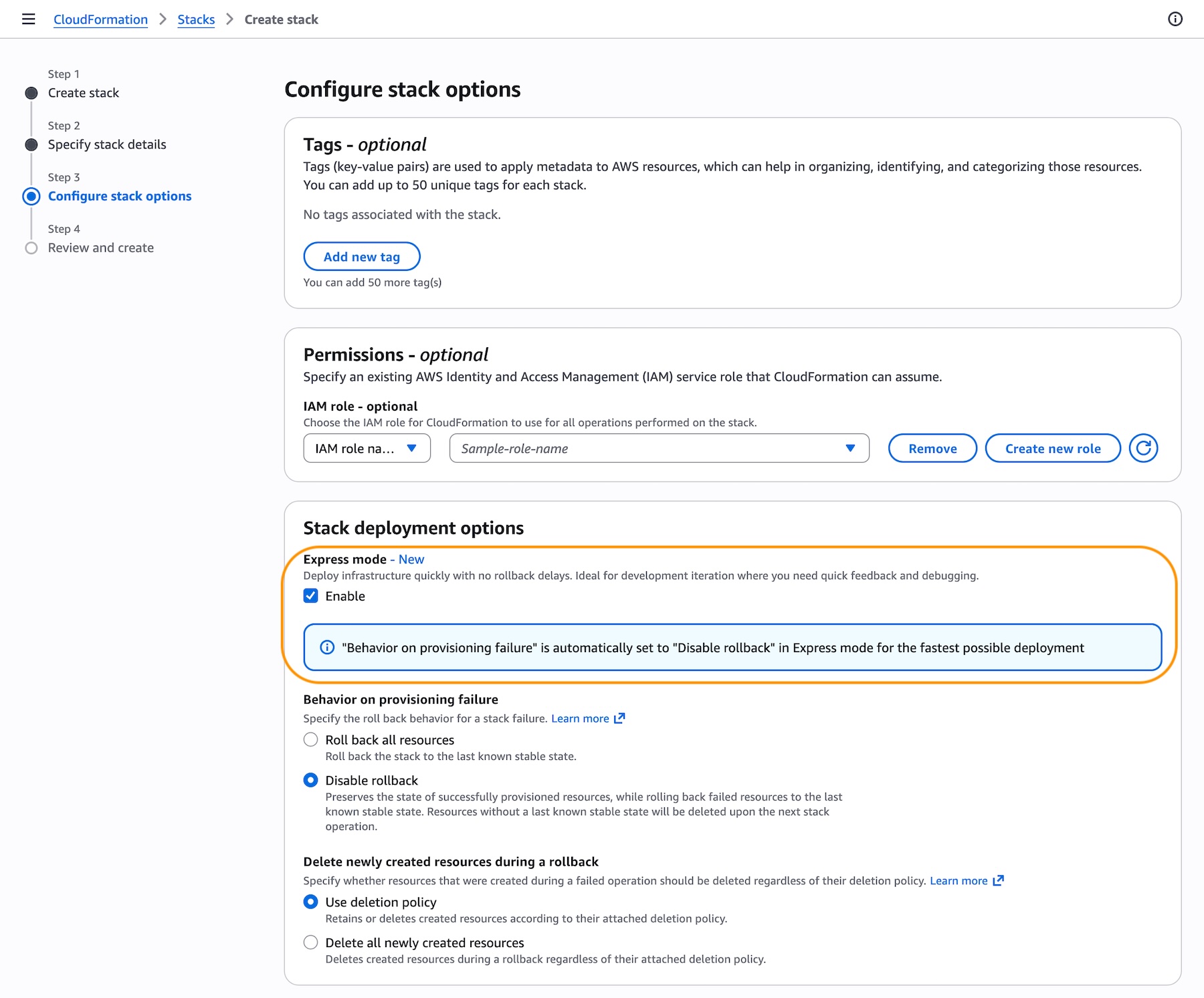

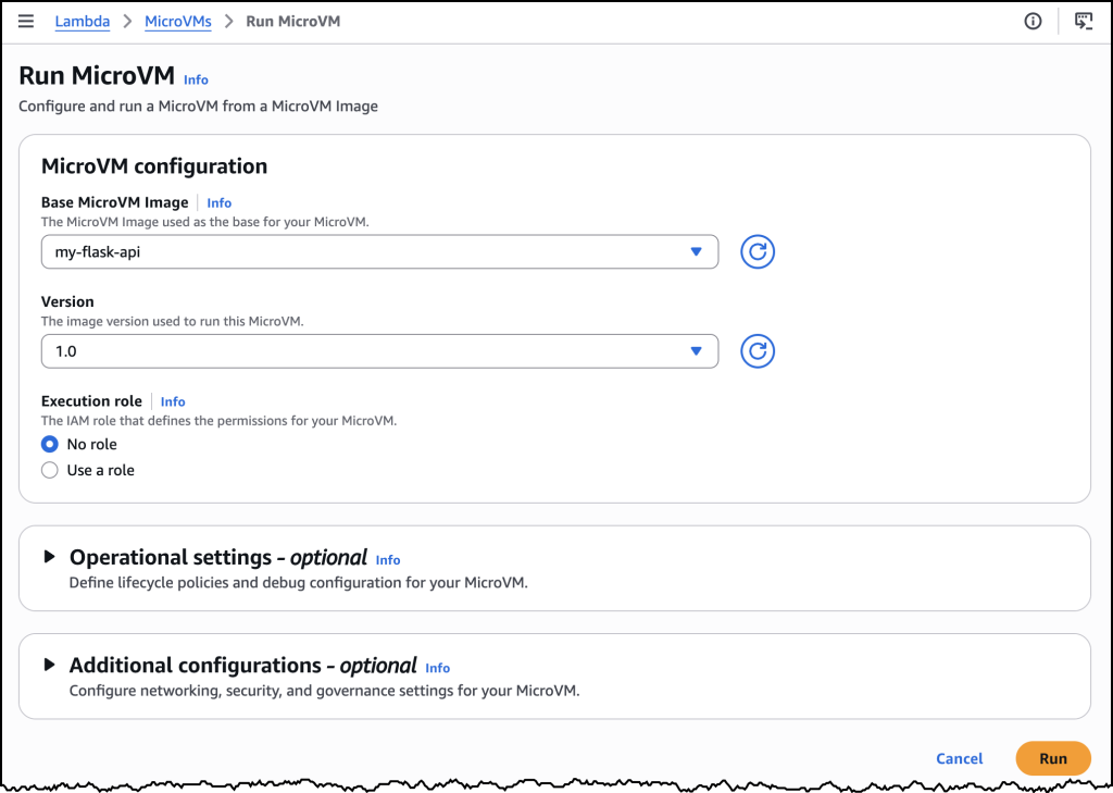
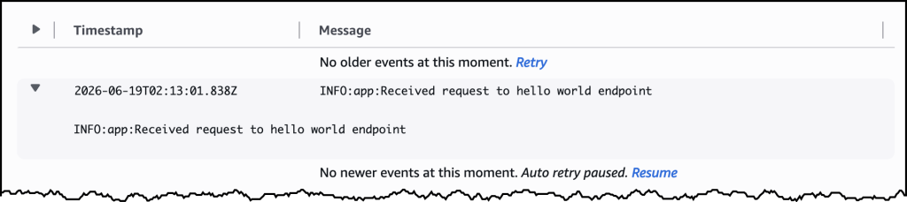
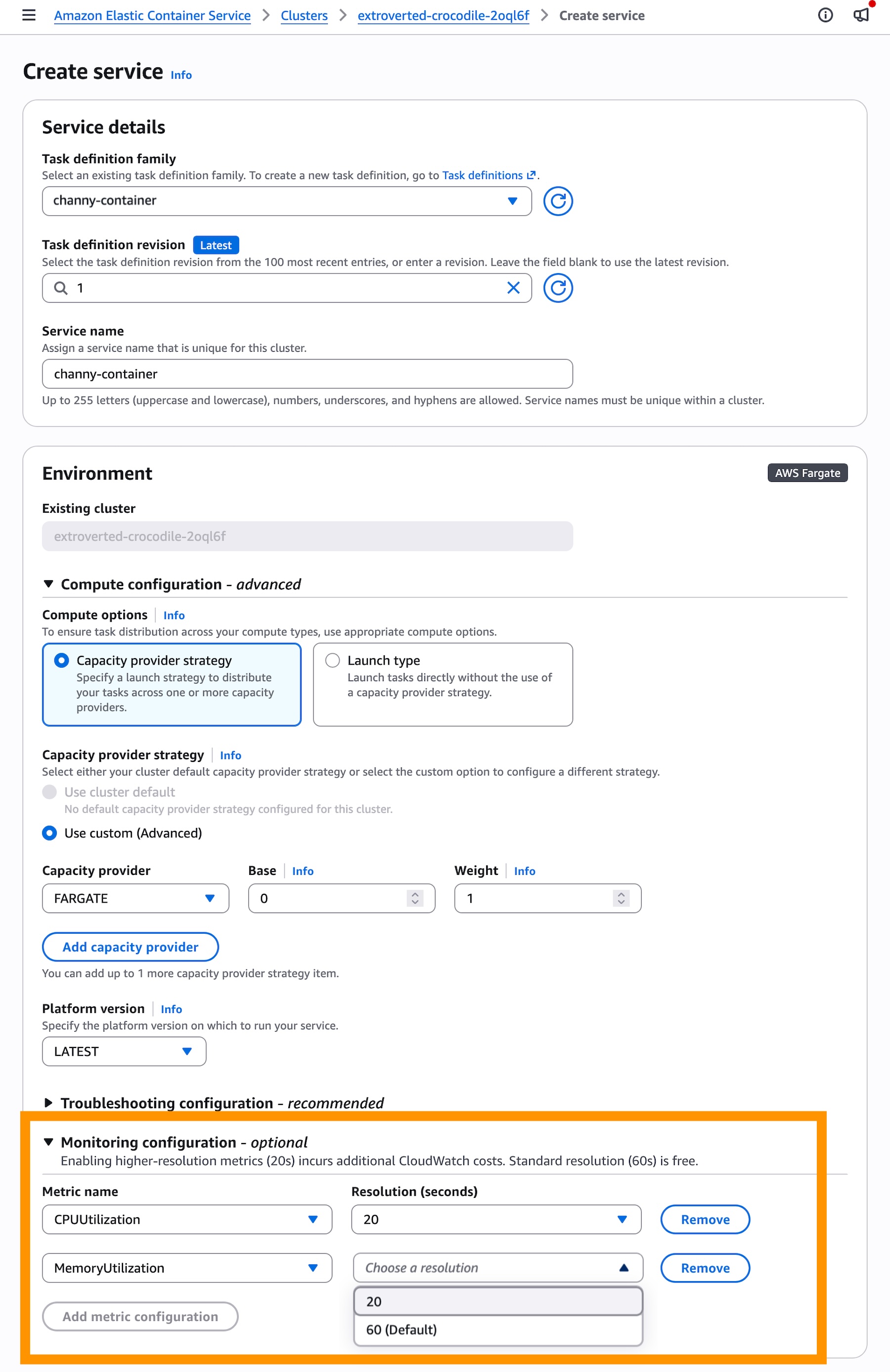
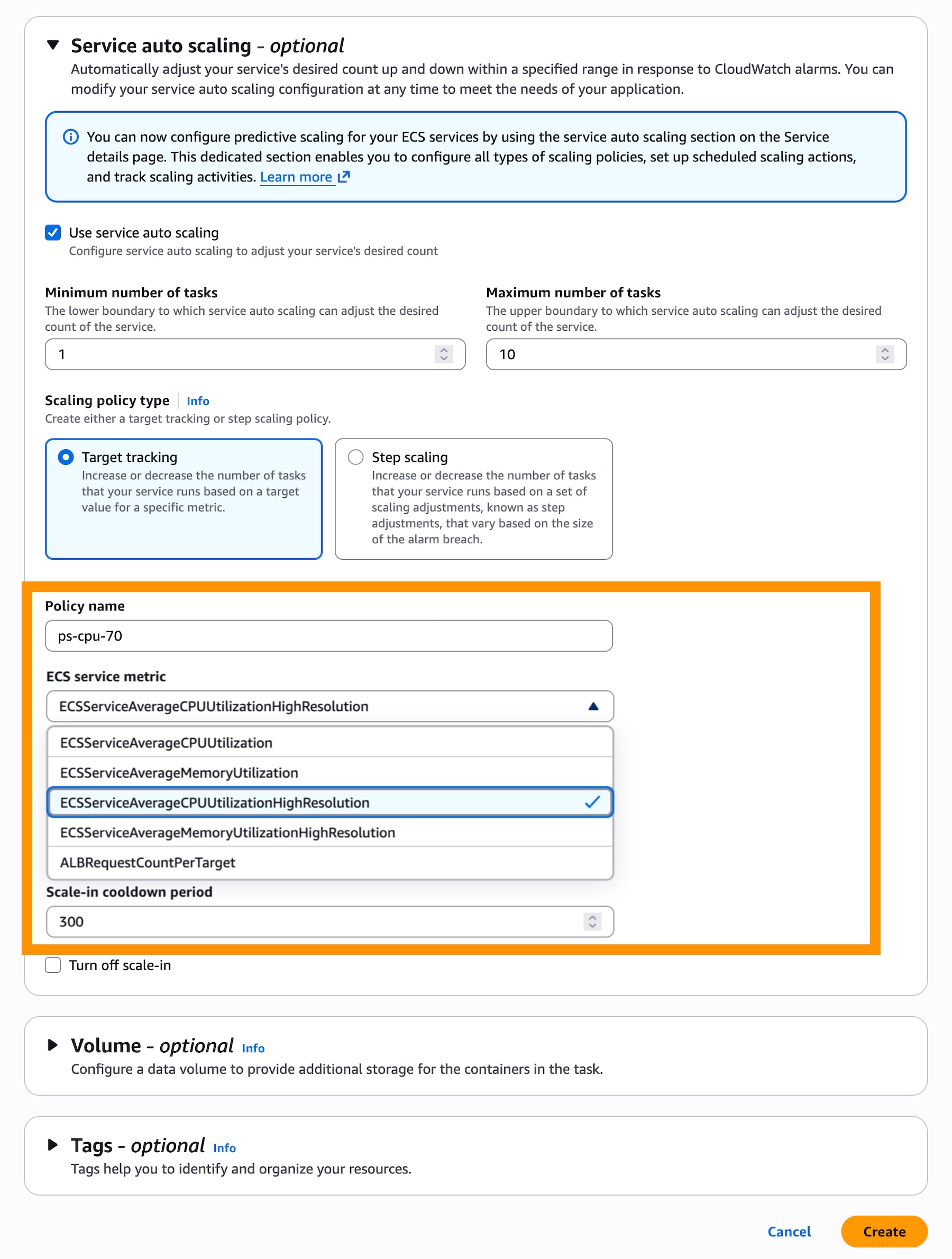
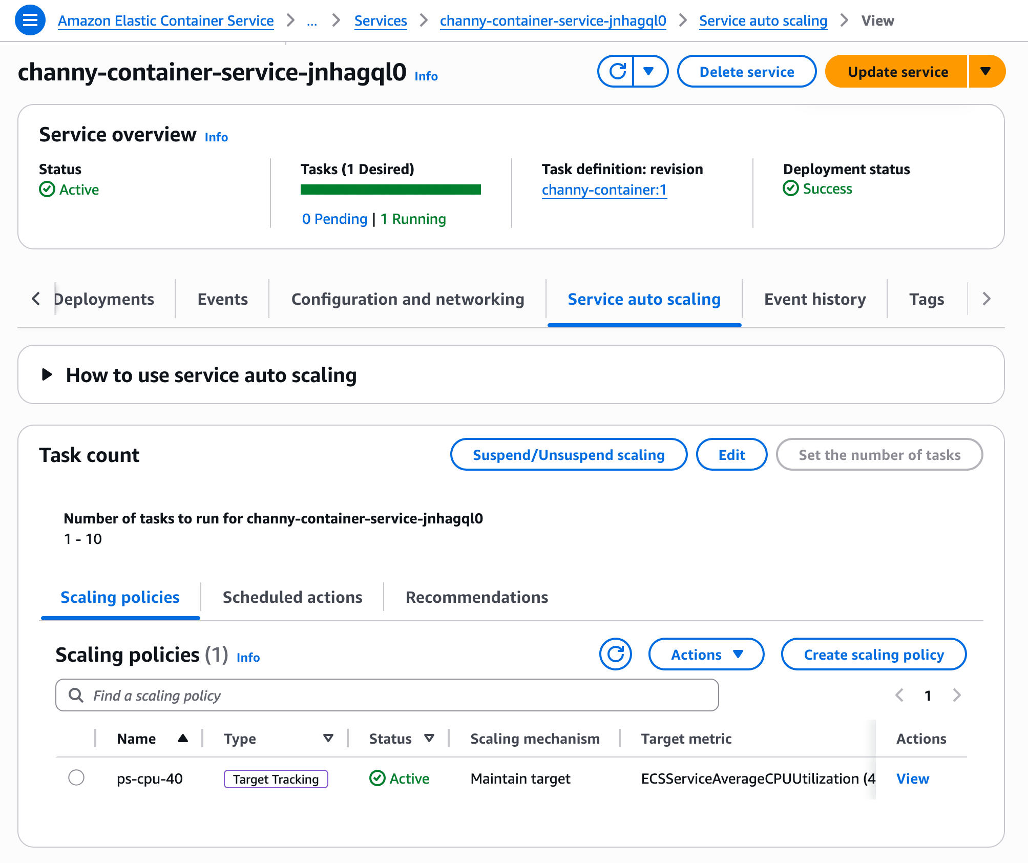
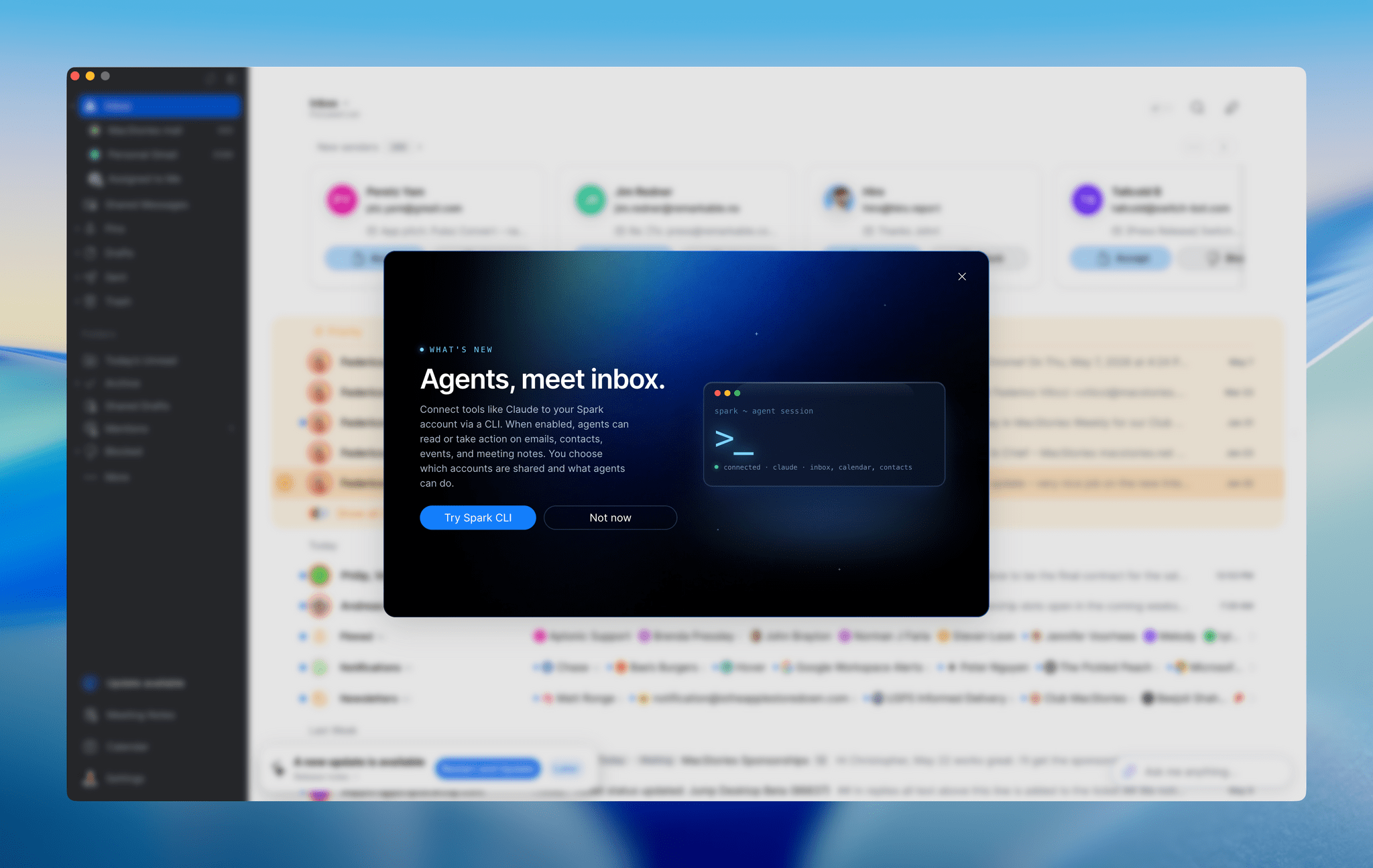
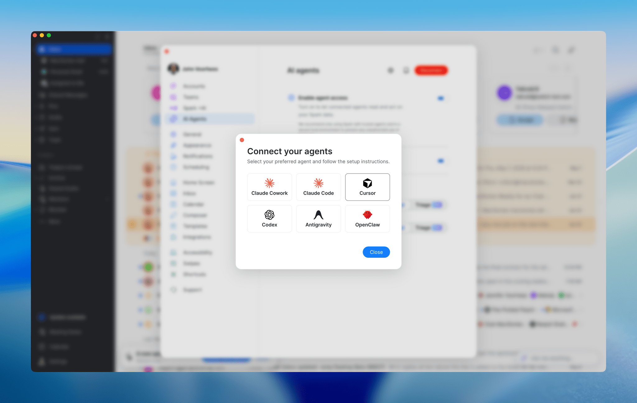
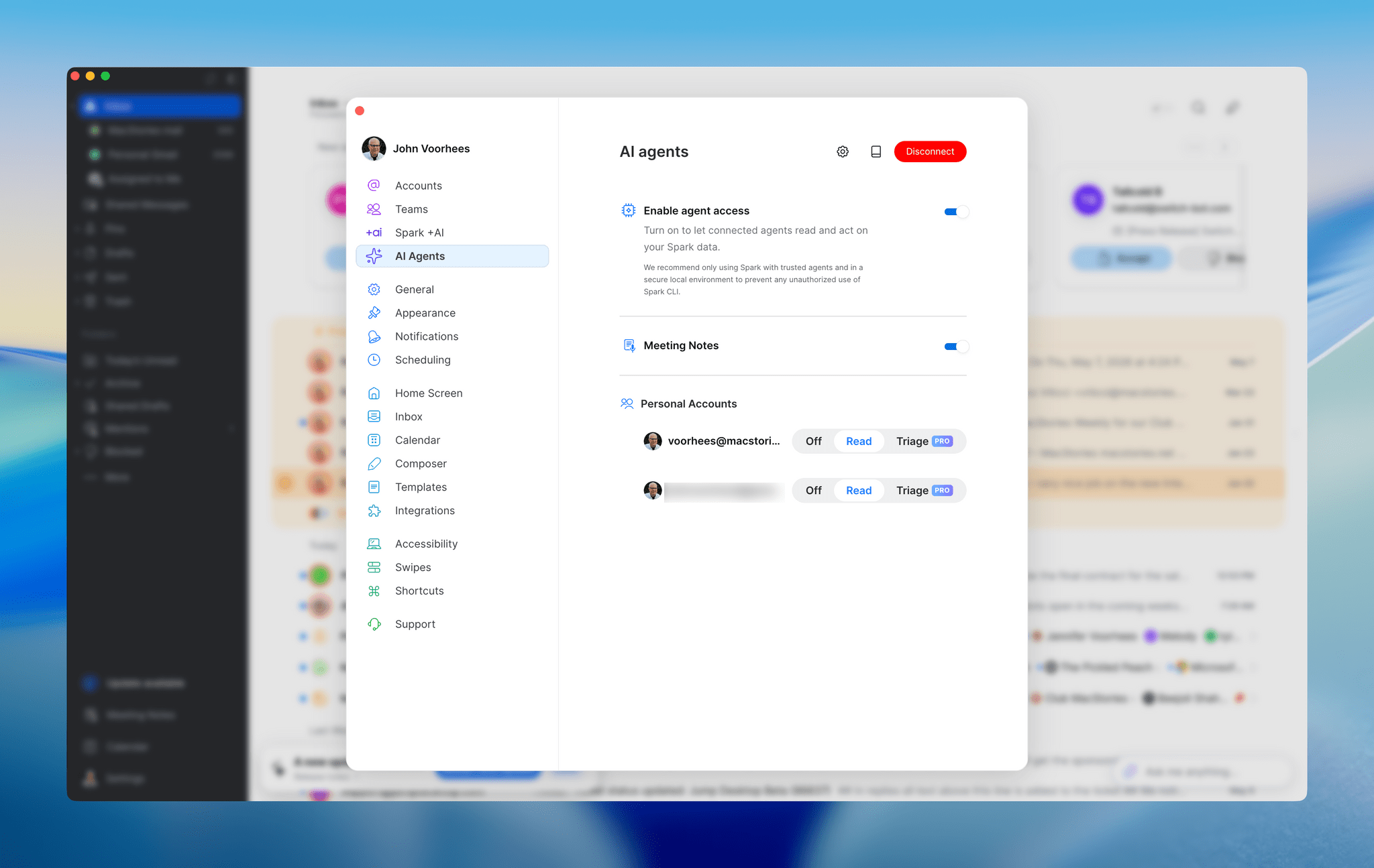
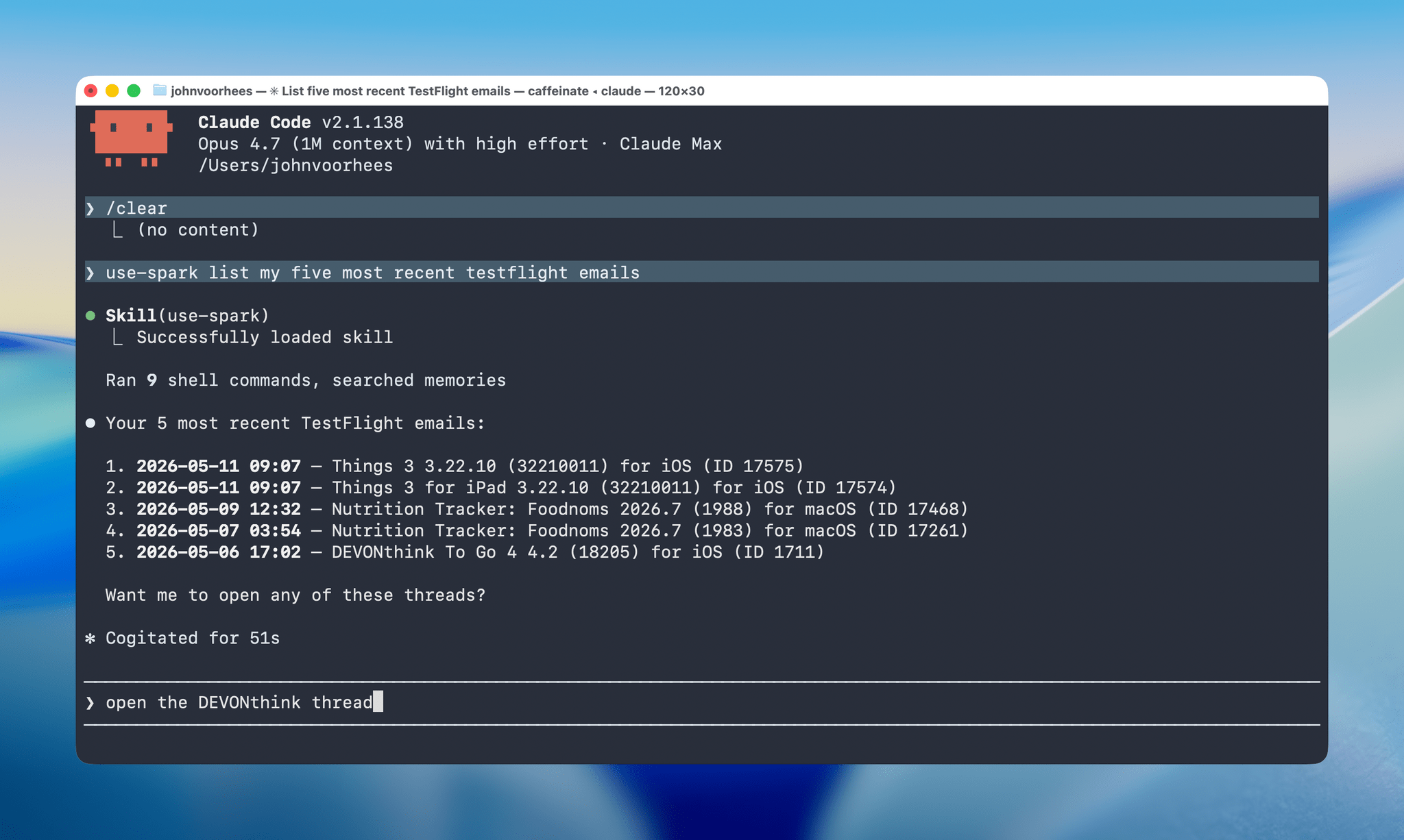
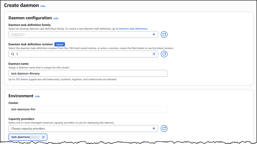


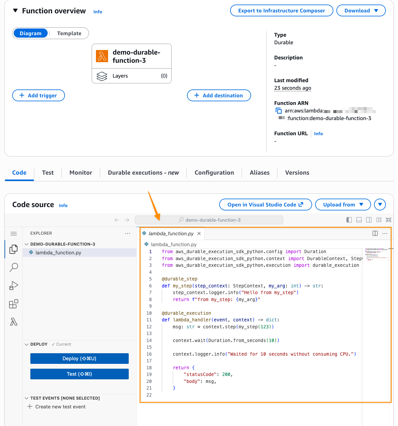
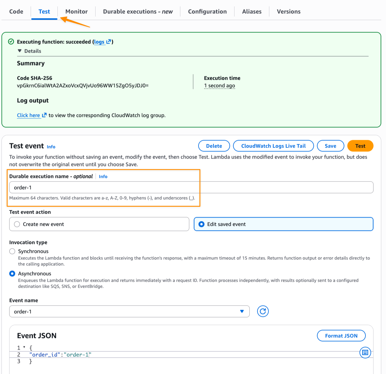
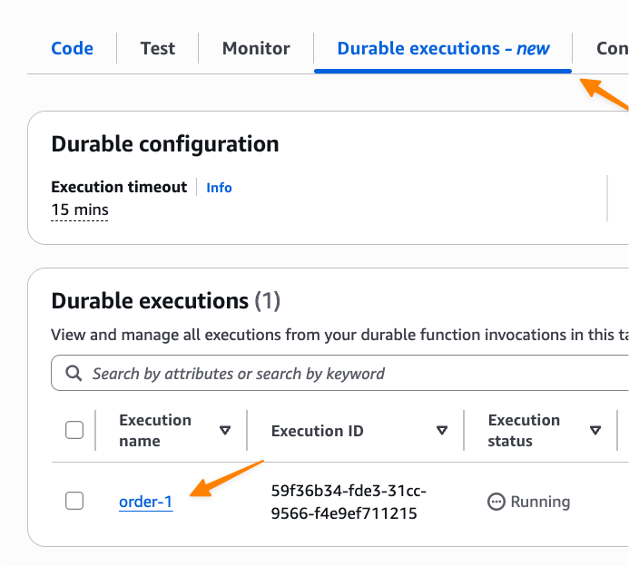
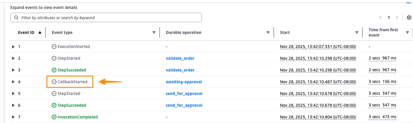
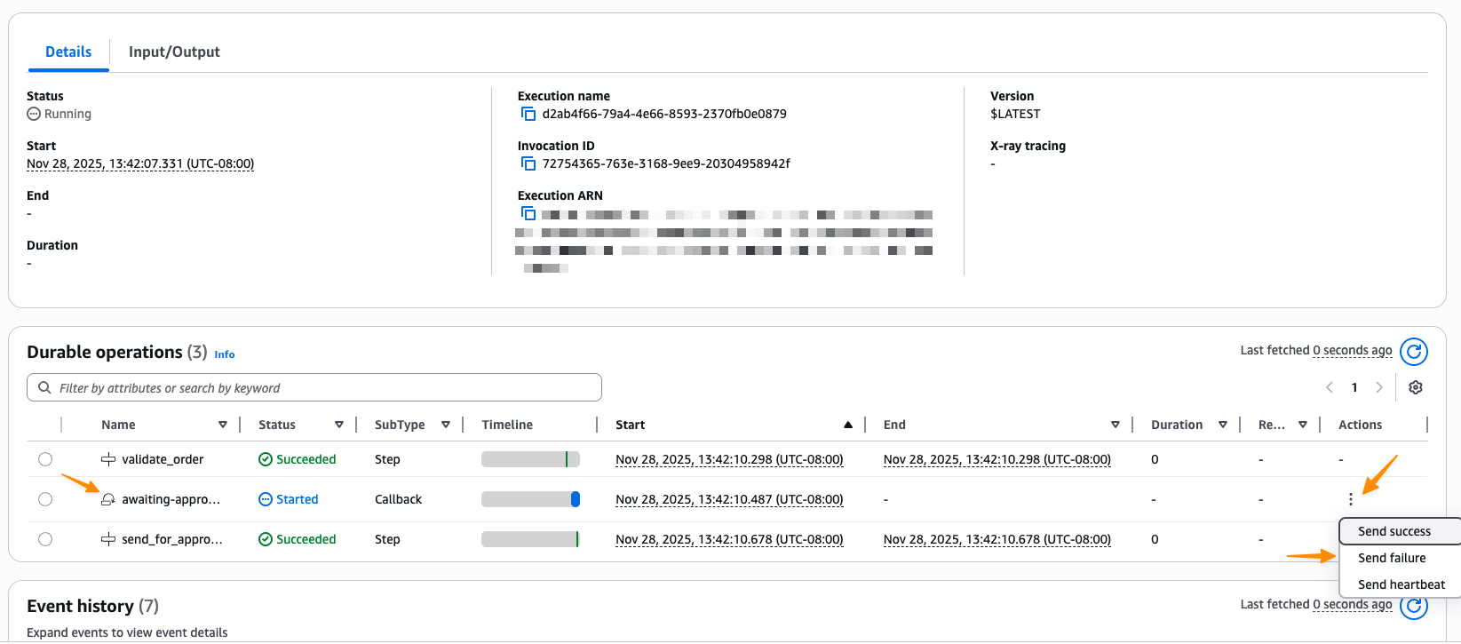
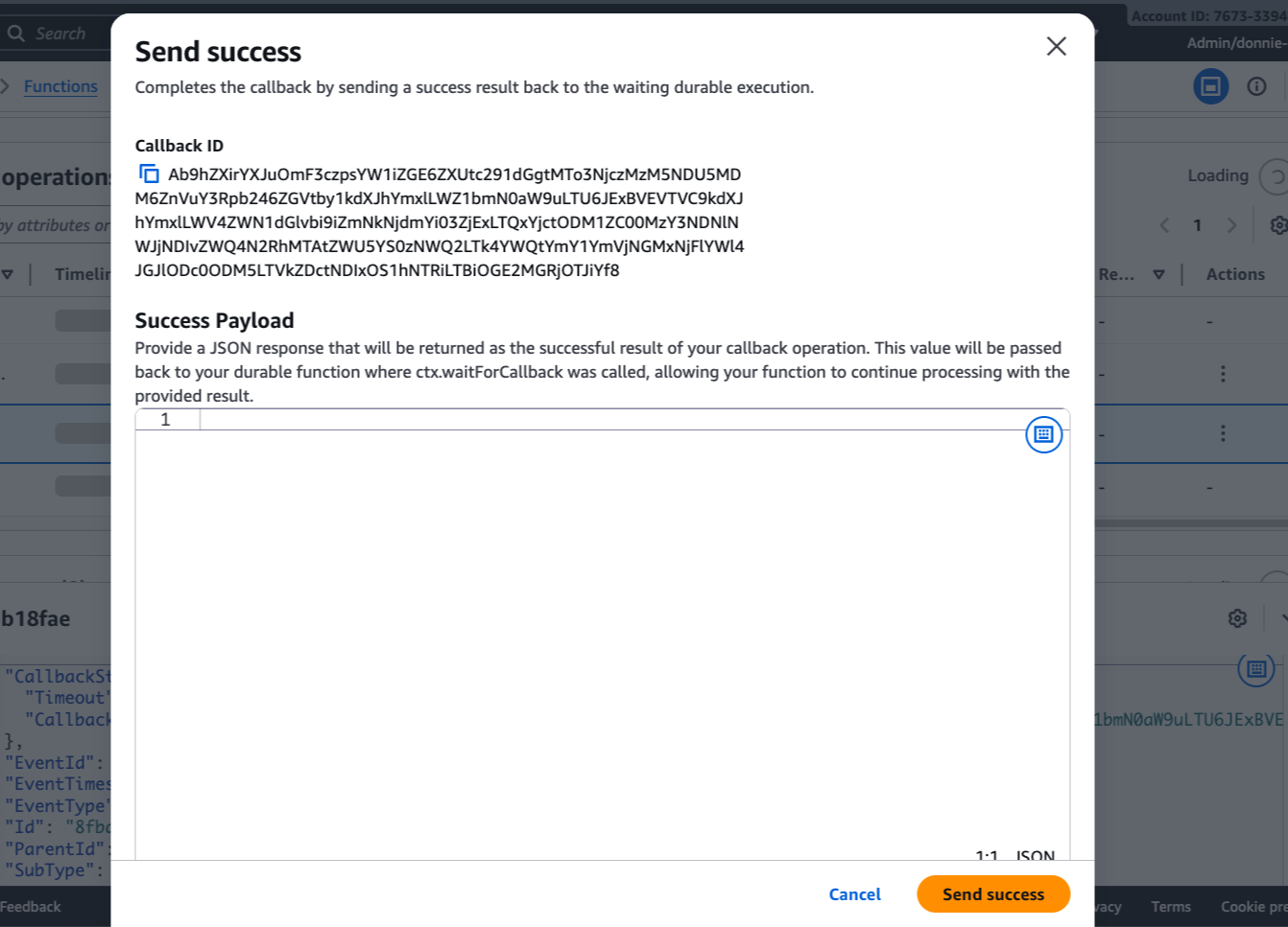
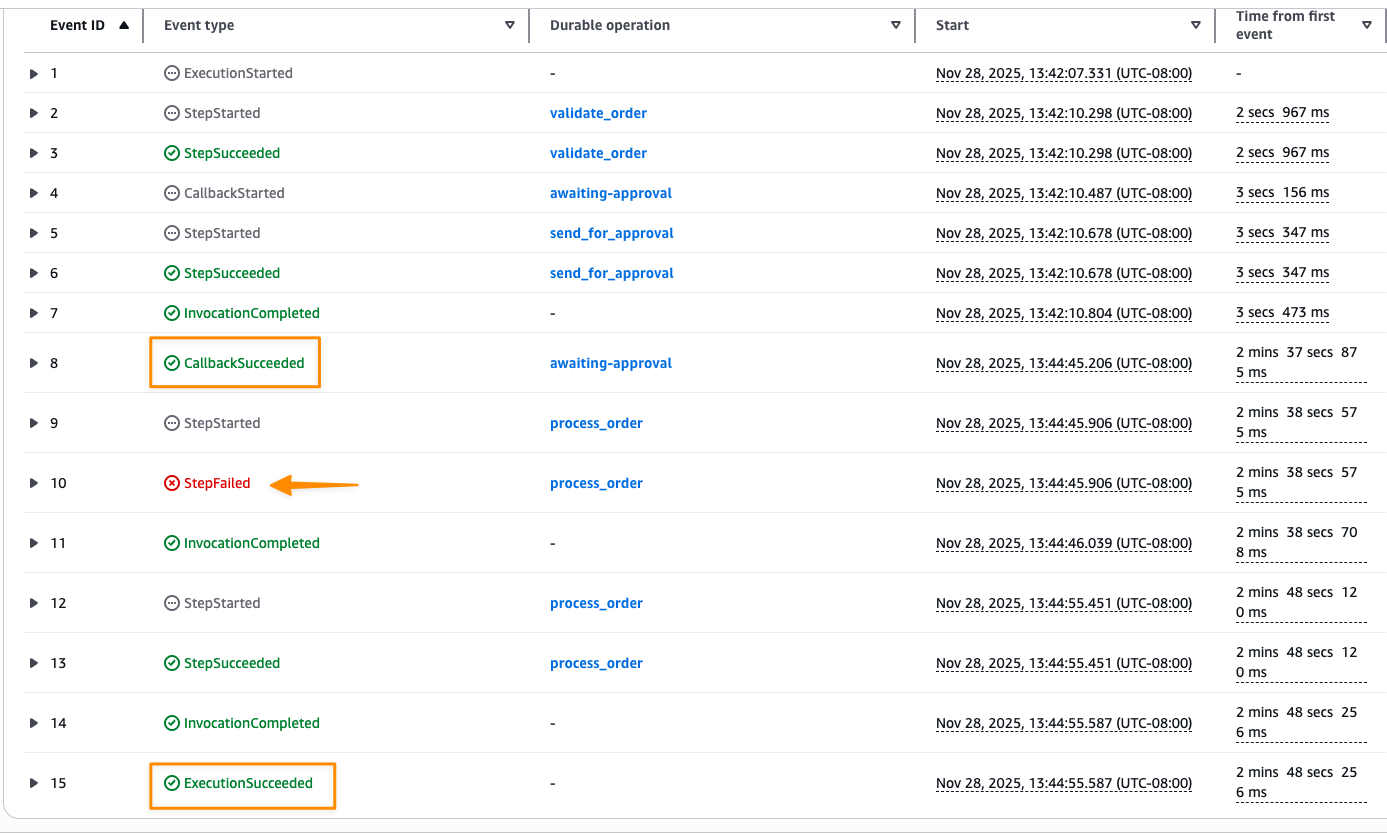
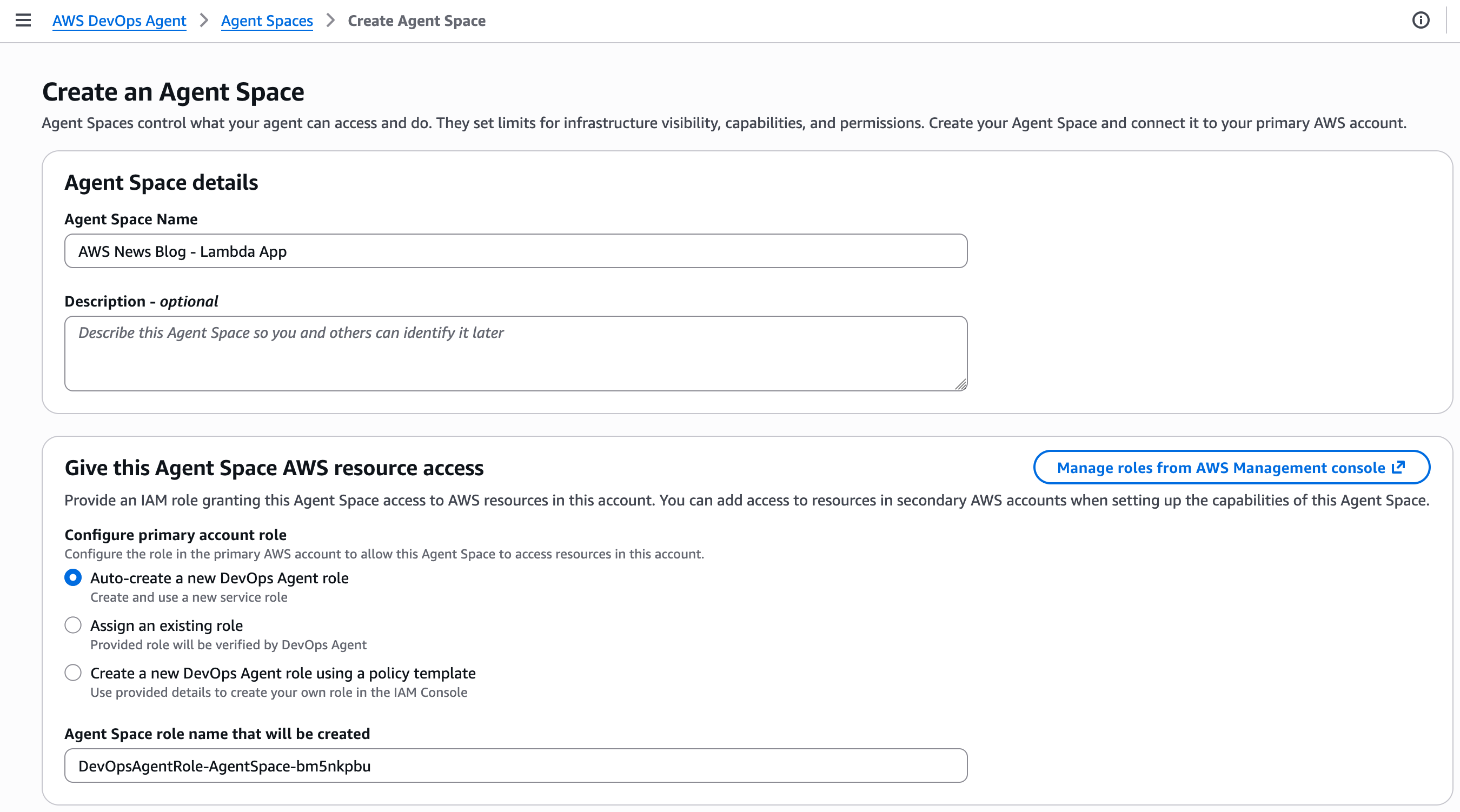
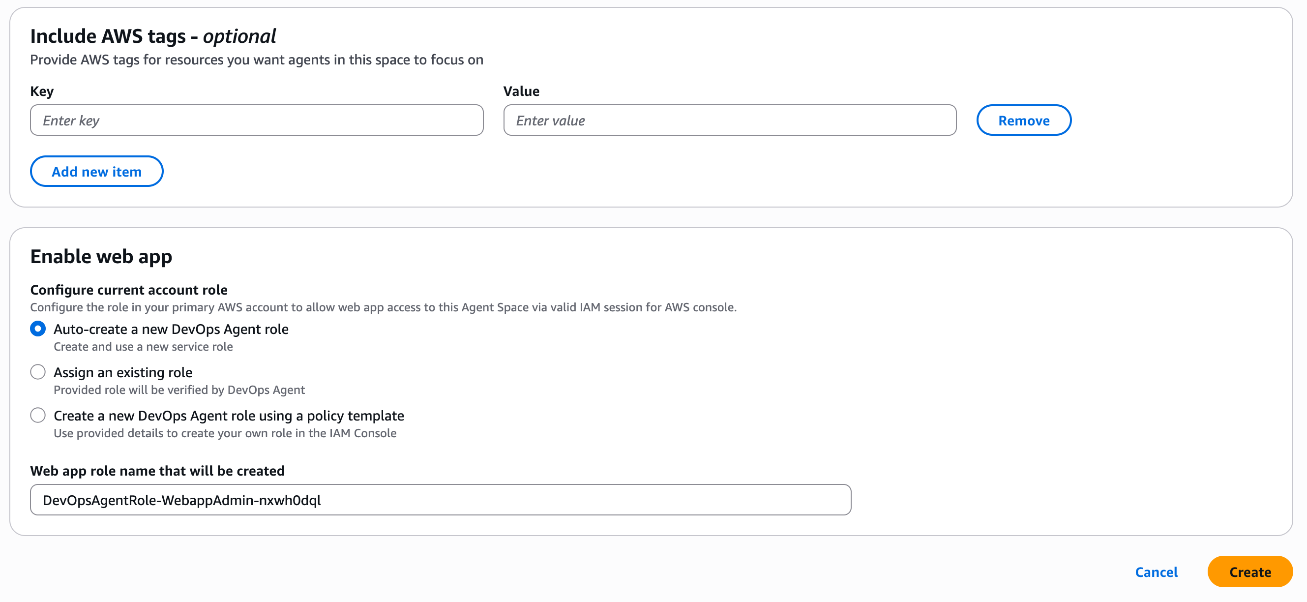
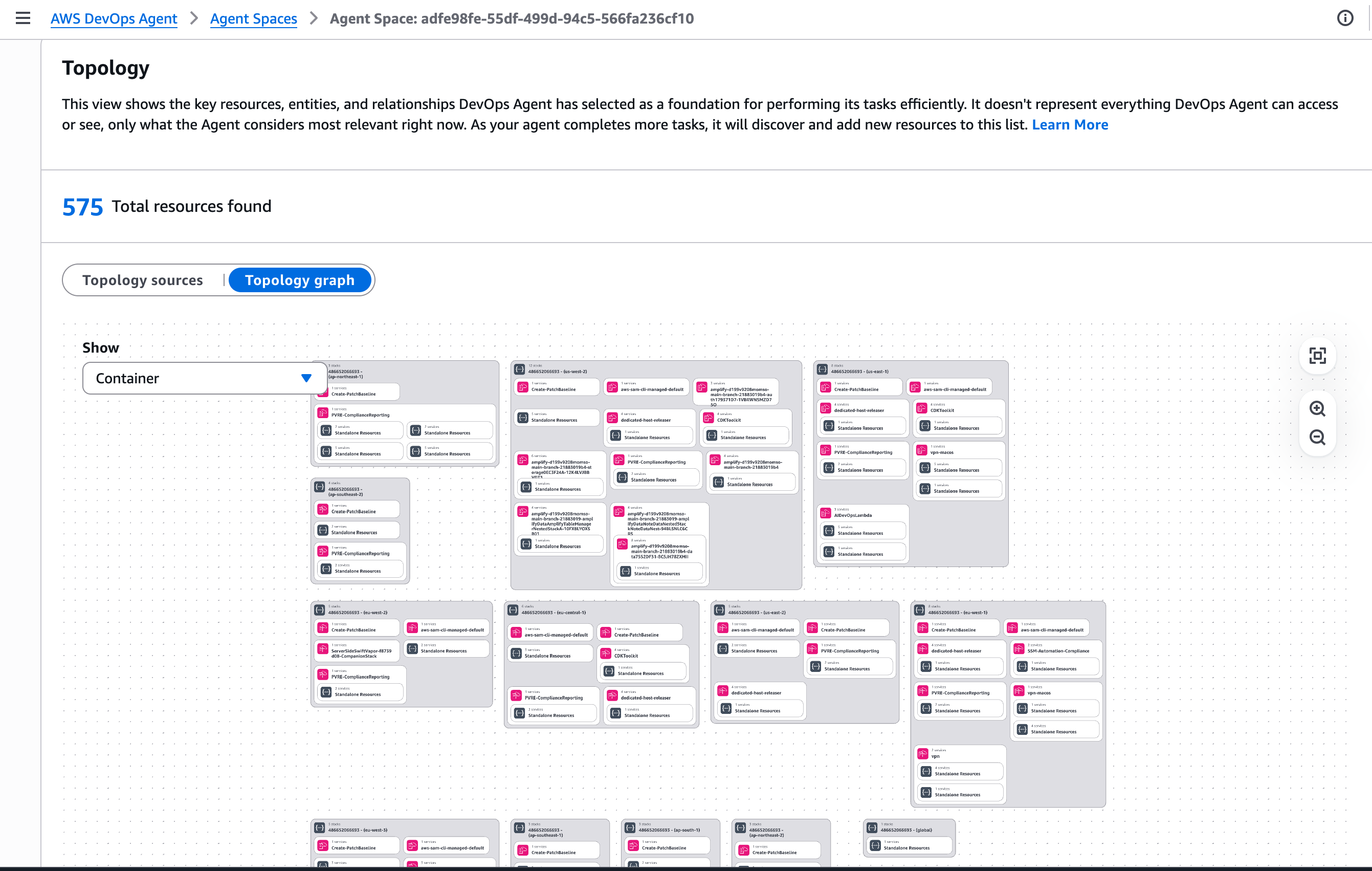
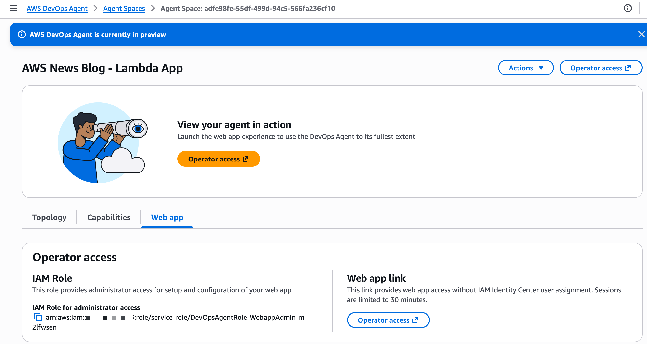
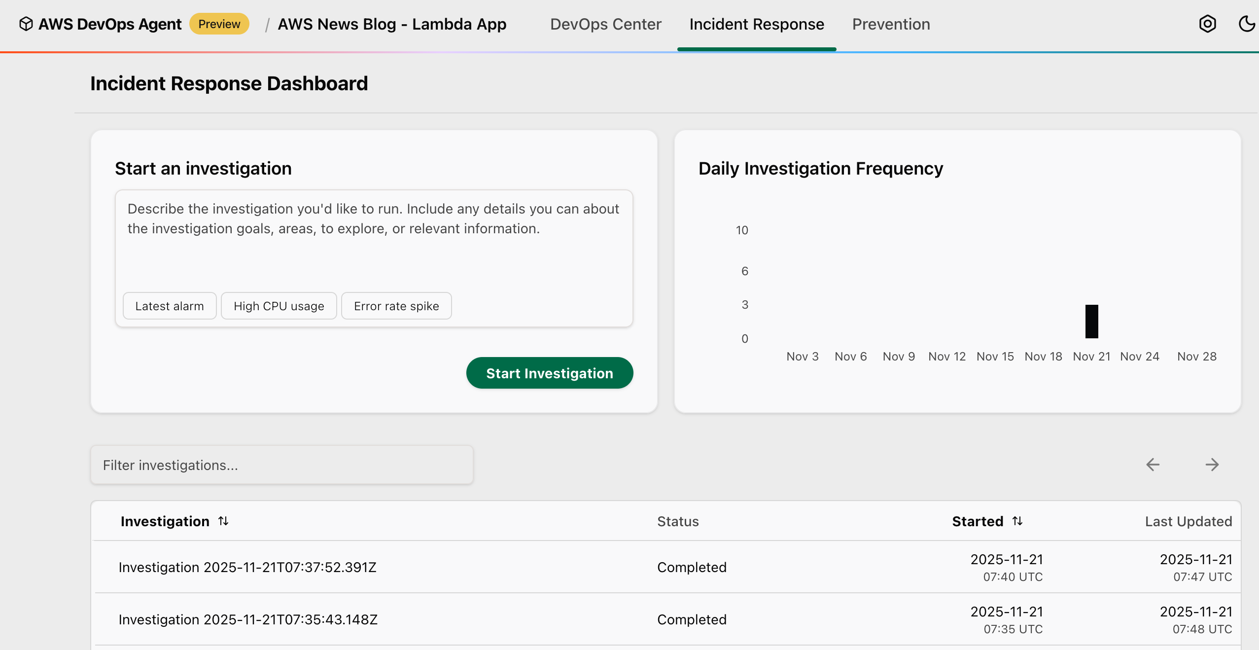
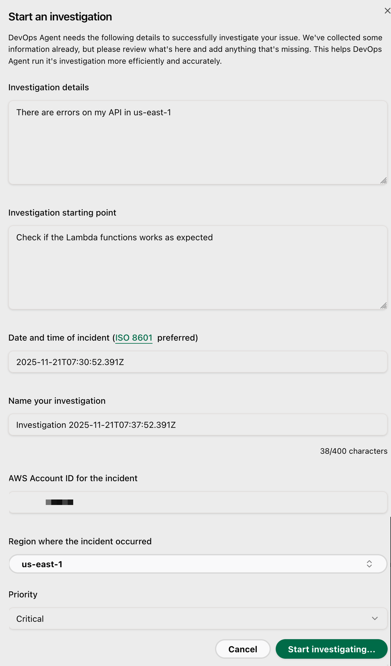
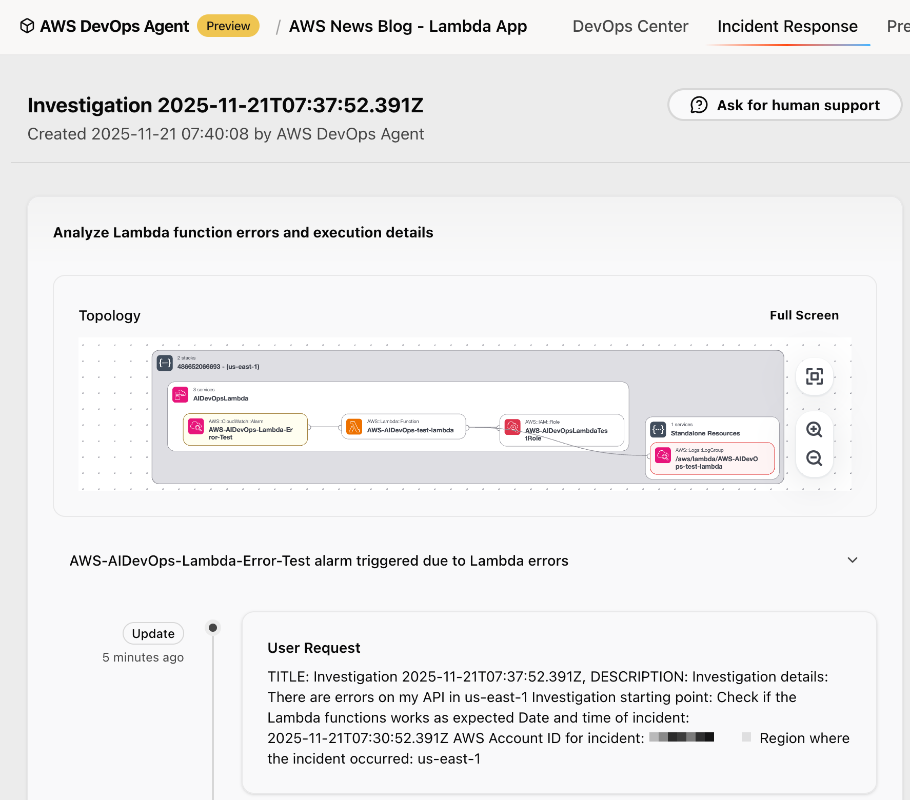
 .
.
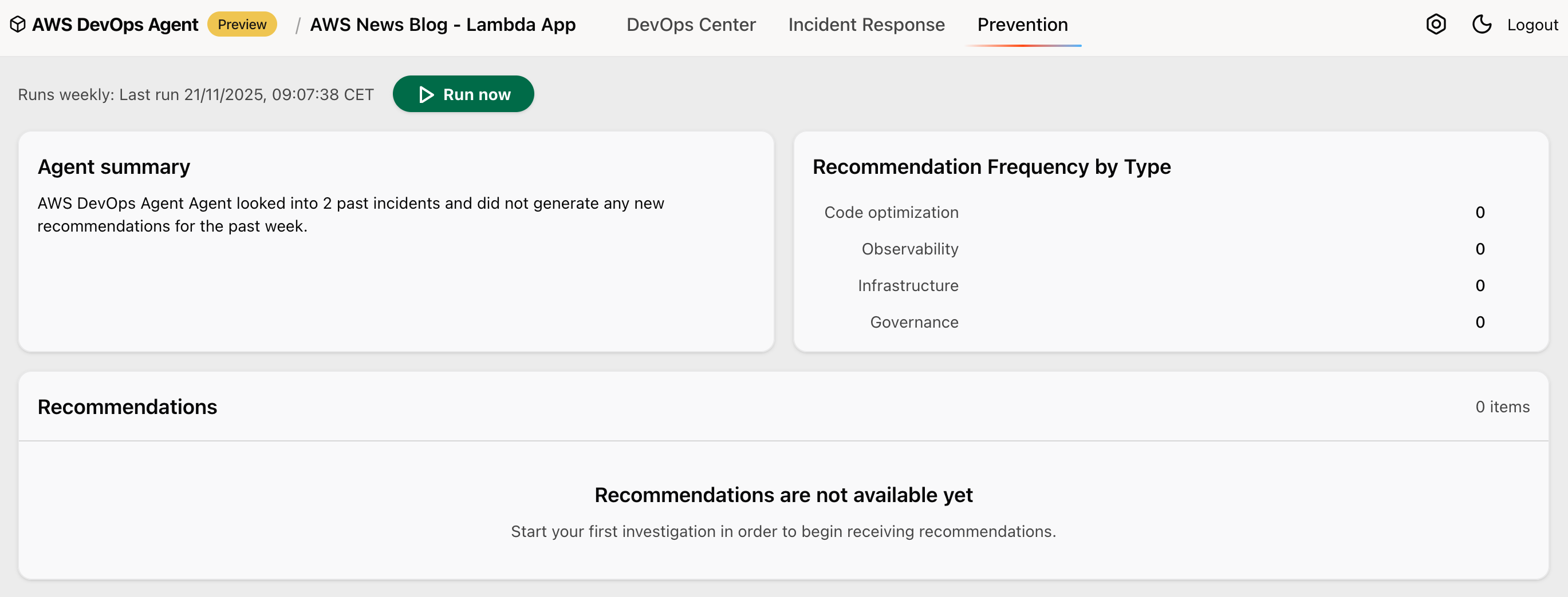
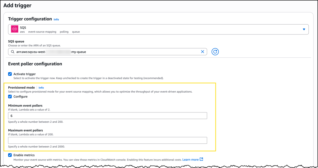
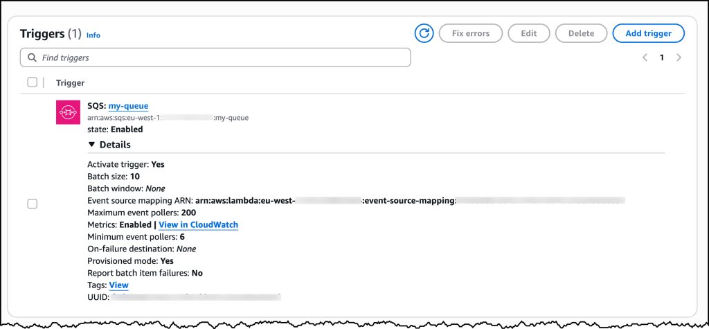


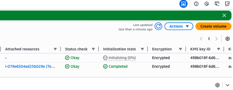


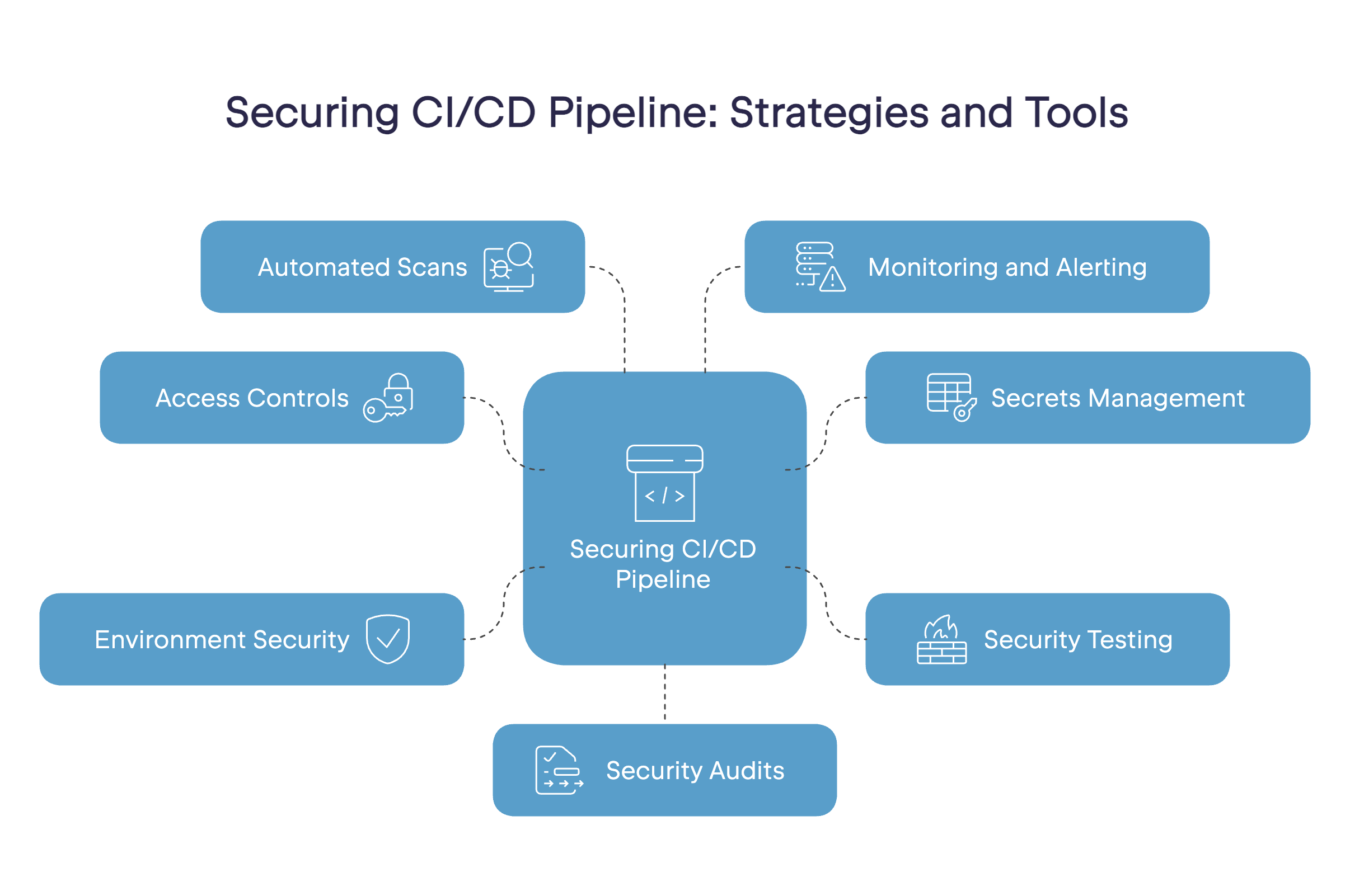
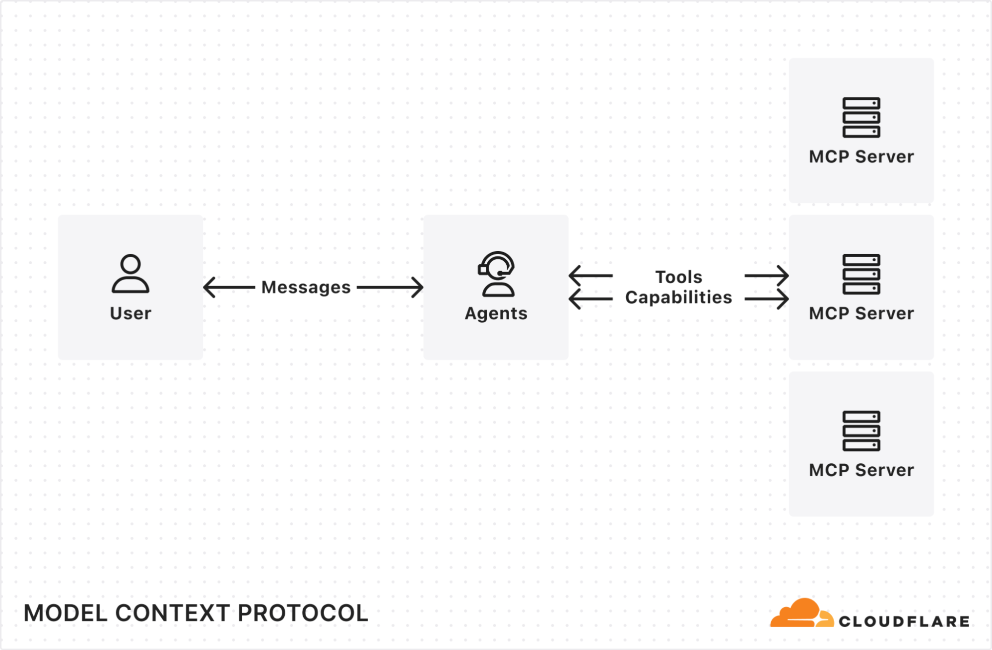
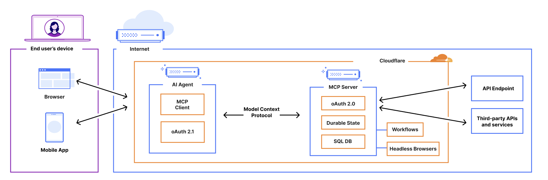
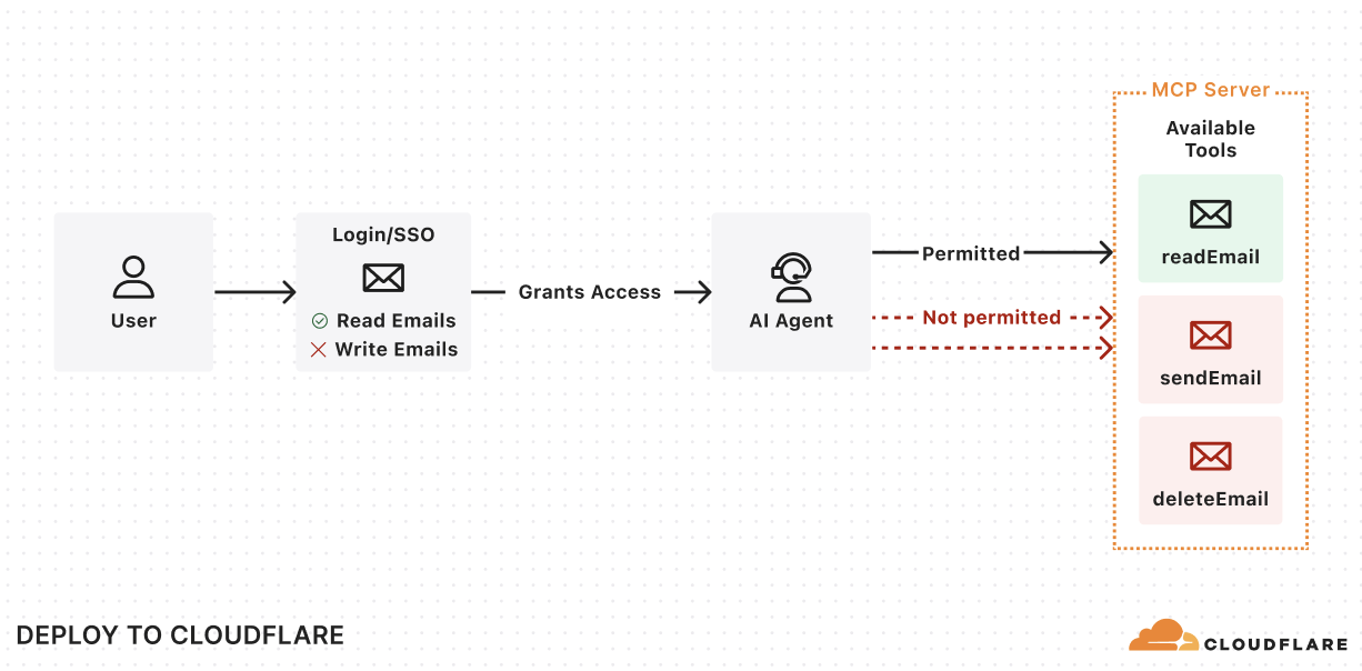
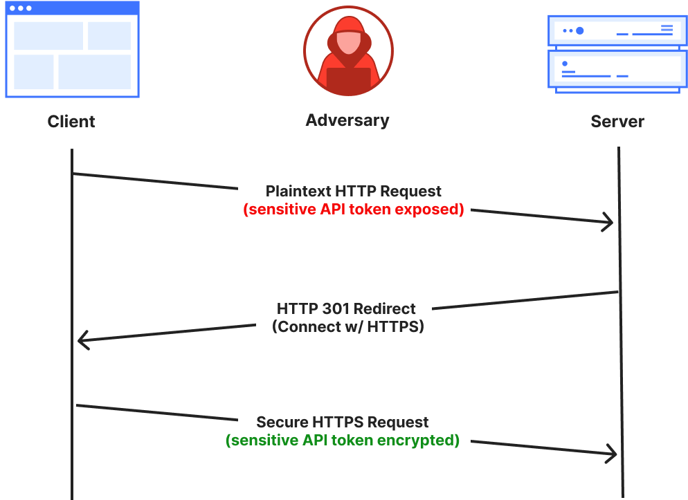
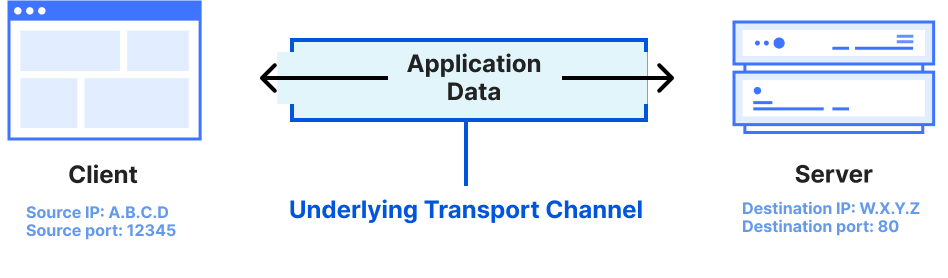
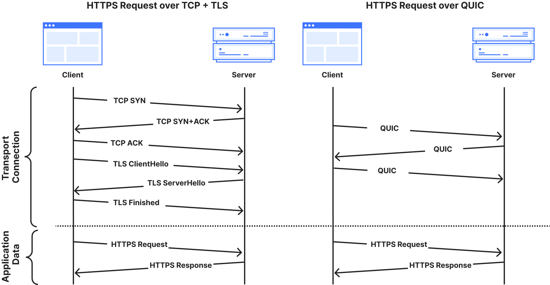
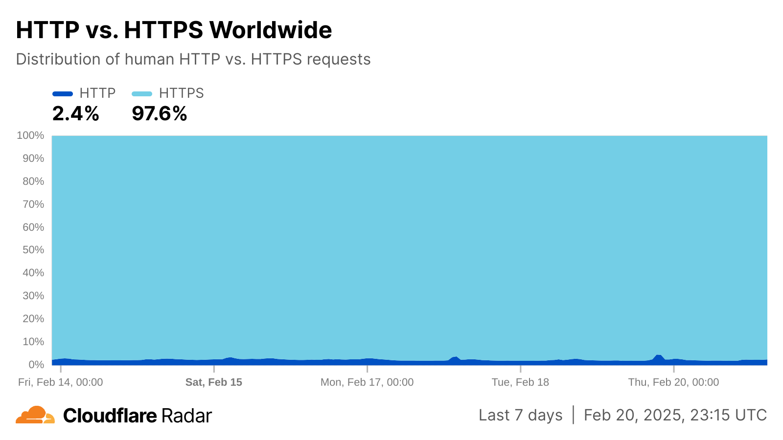


 AWS customers make use of Amazon Simple Storage Service (Amazon S3) at an incredible scale, regularly creating individual buckets that contain billions or trillions of objects! At that scale, finding the objects which meet particular criteria — objects with keys that match a pattern, objects of a particular size, or objects with a specific tag — becomes challenging. Our customers have had to build systems that capture, store, and query for this information. These systems can become complex and hard to scale, and can fall out of sync with the actual state of the bucket and the objects within.


 Taking all of this into account, I am happy to be able to tell you about the new Amazon FSx Intelligent-Tiering storage class, available today for use with


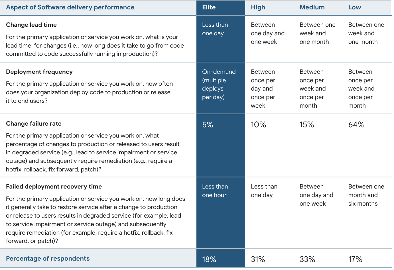
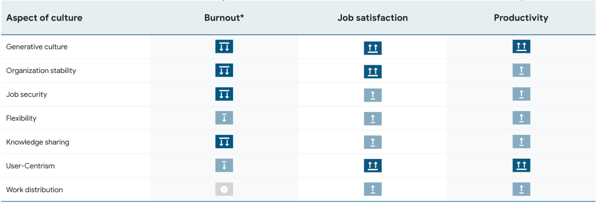
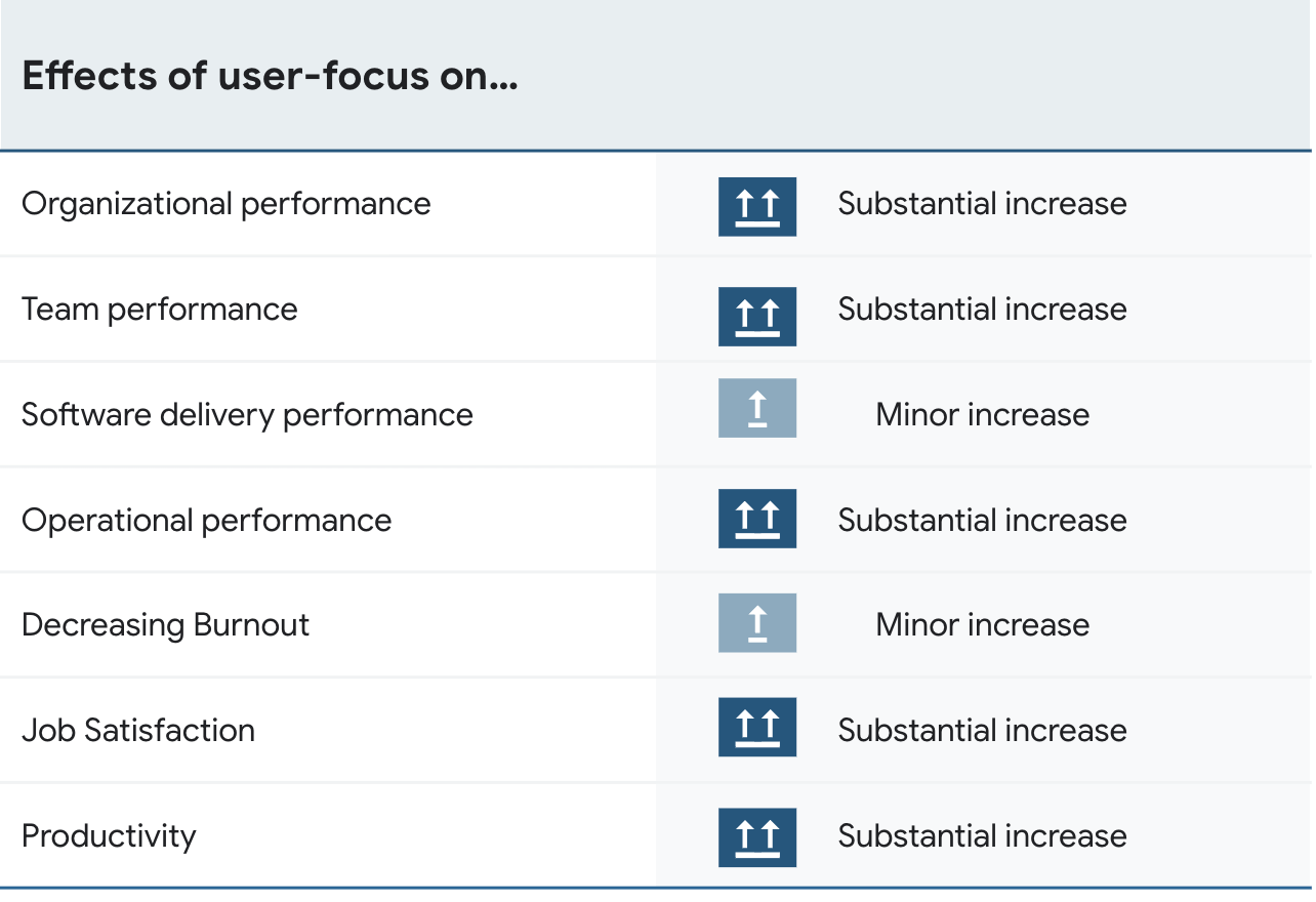
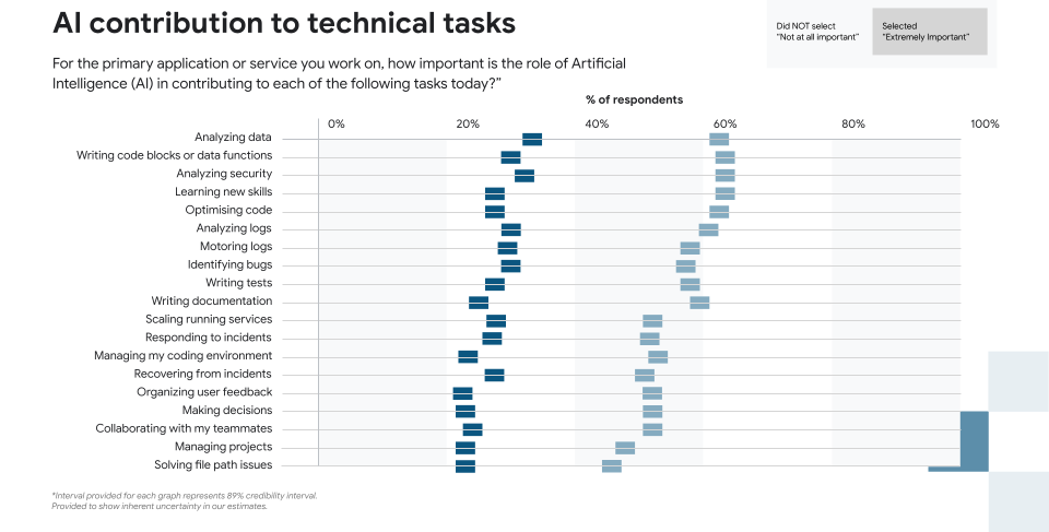


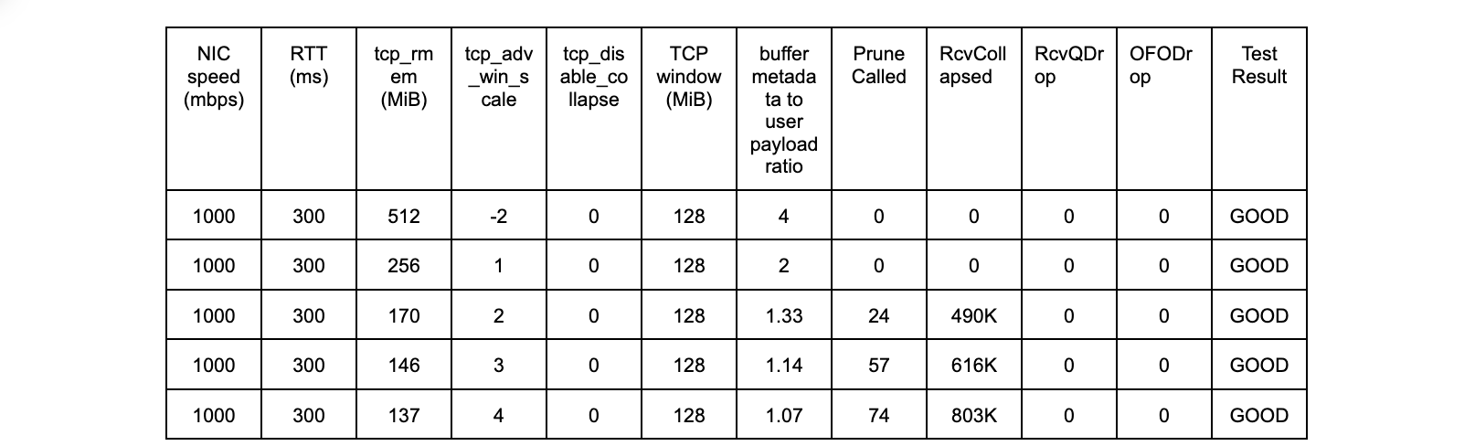
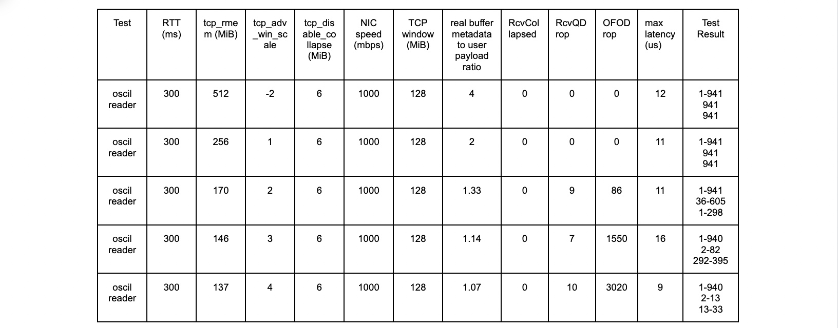
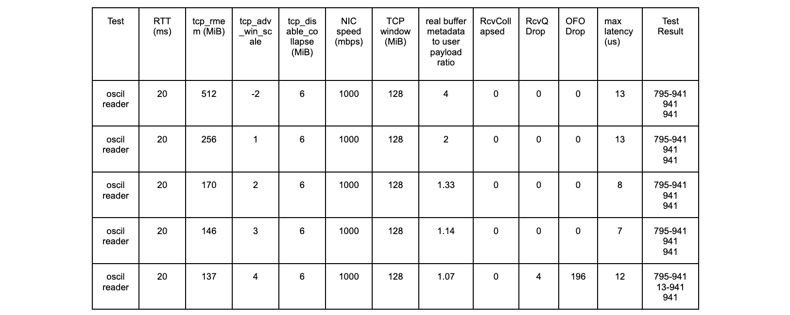
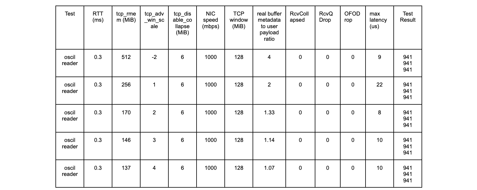
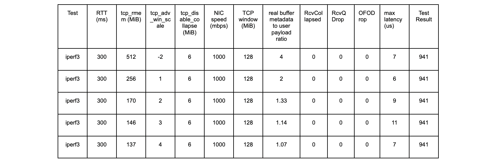
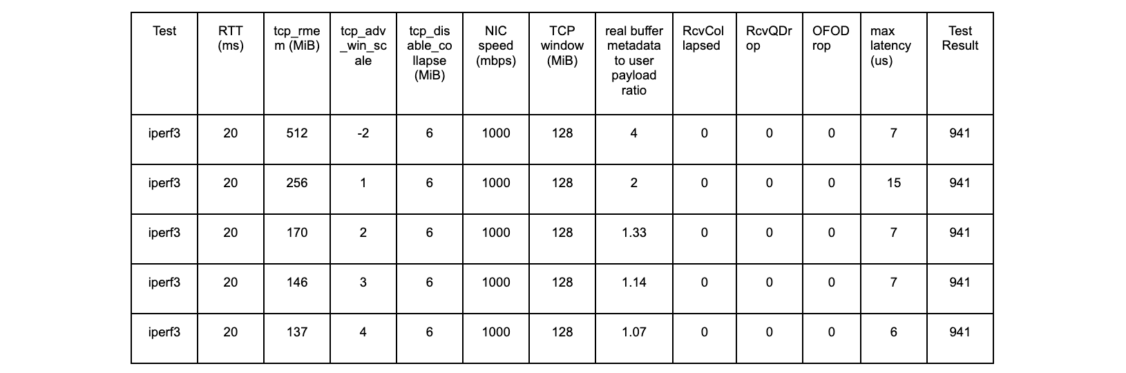
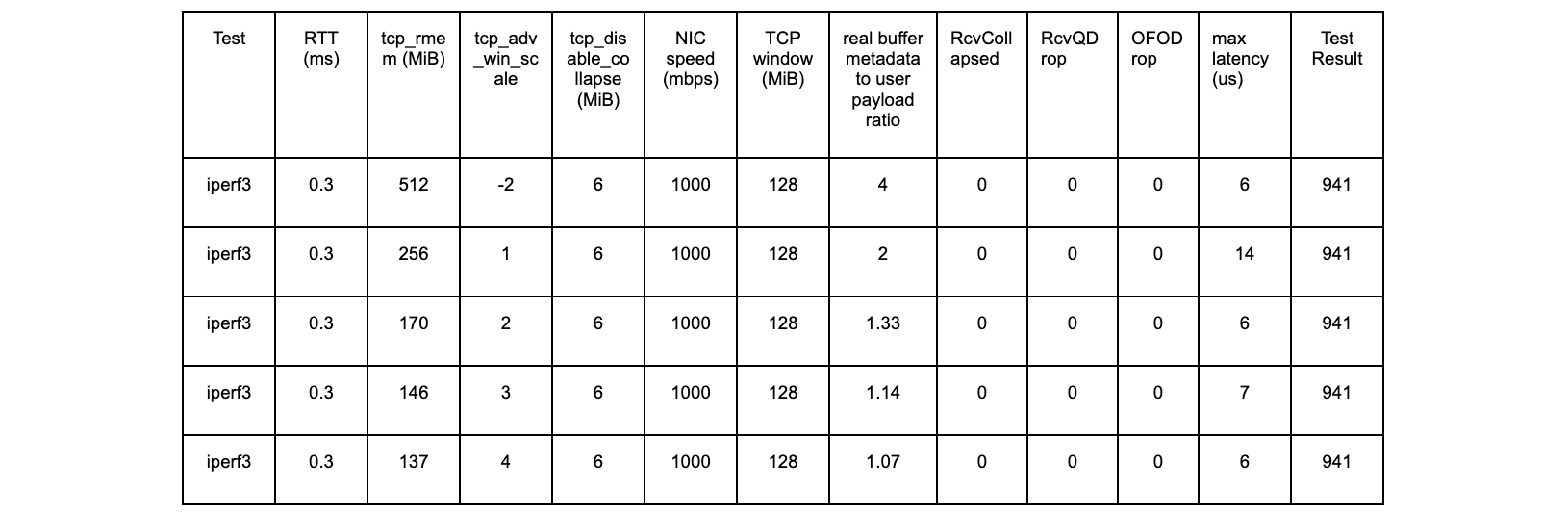
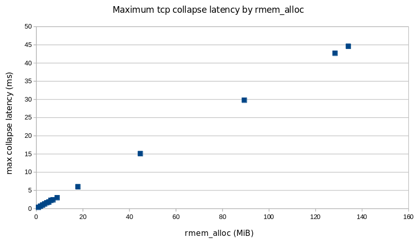
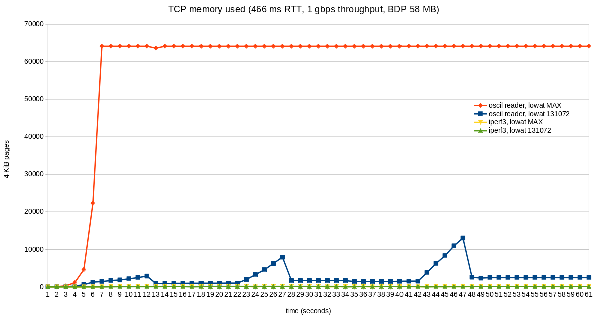


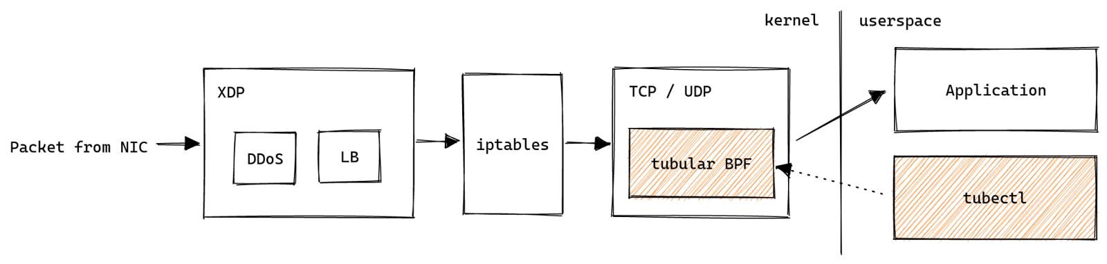

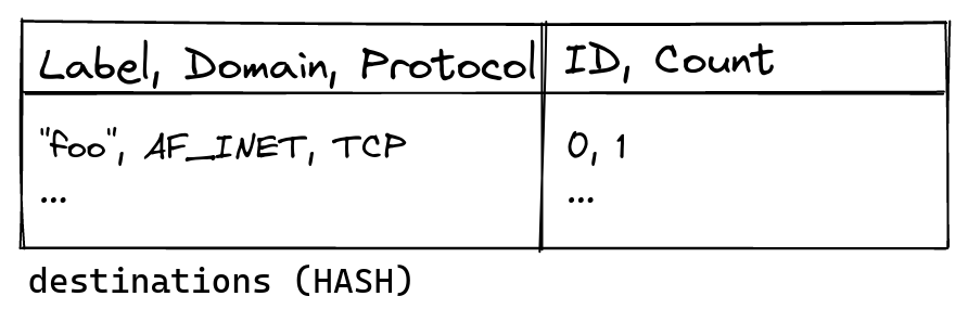
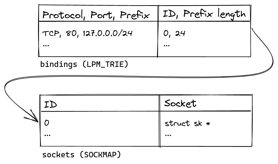


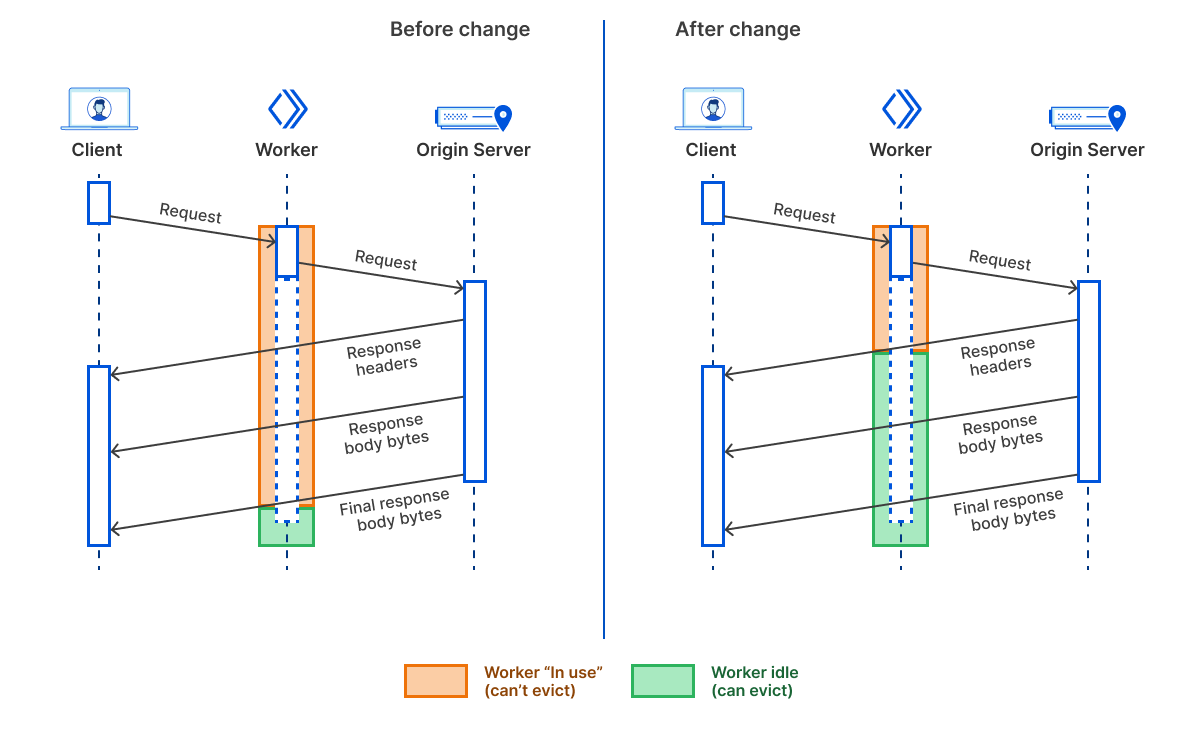


